

Simple Linear Regression: Step 1
You probably remember the concept of simple linear regression intuition from your high school years. It’s the equation that produces a trend line that is sloped across the X-Y axes.
Here’s the simple linear regression equation to refresh your memory:
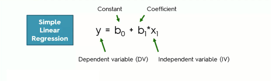
Here’s a breakdown of the simple linear regression equation:
- The dependent variable (DV): As you probably already guessed from the name, the DV is a variable that you try to understand in terms of its dependence on another variable. For example, how is your body fat level affected by the number of hours you spend jogging every week? How does your GPA change in relation to your studying hours?
The body fat level and the GPA here are our dependent variables.
- The independent variable (IV): The IV is the variable that affects the dependent variable. In the two examples that we just mentioned, the jogging hours and the studying hours are the independent variables in their respective cases.
Sometimes, the IV does not have that same sort of direct impact on the DV, though.
- The coefficient: In the simple linear regression equation, the independent variable’s coefficient basically determines how a one-unit change in the IV can affect the DV.
It’s simply the middleman between the DV and the IV. The reason we need this middleman is that the rate of change in the IV can often not be in proportion to the change in the DV.
- The constant (b0): That’s the point where the straight line intersects with the Y-axis.
Let’s take an example so that you can see how all of this actually works.
Example: Salary & Experience
In the example below, the salary is the dependent variable (y), while experience is the independent variable (x1).
In that case, the equation would go like this:
Salary = b0 + b1 * Experience
Using the results, you then go on to draw a straight line that best fits these results.

As we move on to the next tutorial and talk about ordinary squares, you’ll get to understand what exactly is meant by “best fits” in this context.
As you can see, the constant here is 30k. What this means is that when you start off without any experience, the salary starts at $30,000. This is the basic point from which the changes take place.
What number do we use for the coefficient, then?
Since we’re dealing with a sloped line, b1 is the slope of our line. That way the steeper the line the bigger the change that happens to the dependent variable (y) with every unit change in the independent variable (x1).
In this example, b1 is the rate of increase in the salary with every additional year of experience.
If we mark the change on the x-axis (Experience), link it to the straight line, and project that on the y-axis (Salary), we would be able to derive the change in salary.

So, that’s the basic utility of the simple linear regression method. In the next tutorial, we’ll get into more details as to how we can implement it.