The Vanishing Gradient Problem
Today we’re going to jump into a huge problem that exists with RNNs.But fear not!
First of all, it will be clearly explained without digging too deep into the mathematical terms. And what’s even more important – we will discuss the solution to this problem in our next article from the deep learning series.
So, what is this problem called vanishing gradient?
People Behind RNNs
The problem of the vanishing gradient was first discovered by Sepp (Joseph) Hochreiter back in 1991. Sepp is a genius scientist and one of the founding people, who contributed significantly to the way that we use RNNs and LSTMs today.
The second person is Yoshua Bengio, a professor at the University of Montreal. He also discovered the vanishing descent problem but a bit later – he wrote about it in 1994. Yoshua is another person pushing the envelope in the space of deep learning and RNNs, in particular.
If you check his profile at the University of Montreal, you will find that he has contributed to over 500 research papers!
This is just to give you a quick idea, who are these people behind the RNN advancements.
Now, let’s proceed to the vanishing gradient problem itself.
Explaining the Vanishing Gradient Problem
As you remember, the gradient descent algorithm finds the global minimum of the cost function that is going to be an optimal setup for the network.
As you might also recall, information travels through the neural network from input neurons to the output neurons, while the error is calculated and propagated back through the network to update the weights.
It works quite similarly for RNNs, but here we’ve got a little bit more going on.
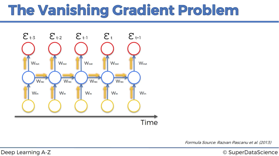
- Firstly, information travels through time in RNNs, which means that information from previous time points is used as input for the next time points.
- Secondly, you can calculate the cost function, or your error, at each time point.
Basically, during the training, your cost function compares your outcomes (red circles on the image below) to your desired output.
As a result, you have these values throughout the time series, for every single one of these red circles.

Let’s focus on one error term et.
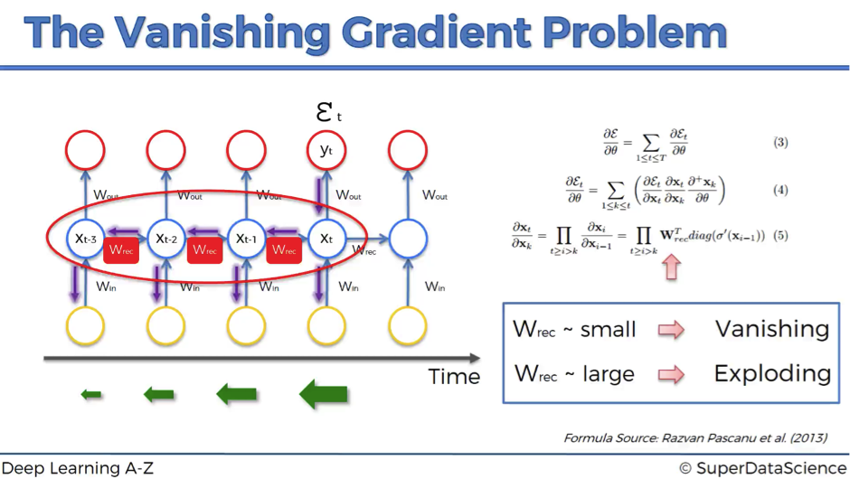
You’ve calculated the cost function et, and now you want to propagate your cost function back through the network because you need to update the weights.
Essentially, every single neuron that participated in the calculation of the output, associated with this cost function, should have its weight updated in order to minimize that error. And the thing with RNNs is that it’s not just the neurons directly below this output layer that contributed but all of the neurons far back in time. So, you have to propagate all the way back through time to these neurons.
The problem relates to updating wrec (weight recurring) – the weight that is used to connect the hidden layers to themselves in the unrolled temporal loop.
For instance, to get from xt-3 to xt-2 we multiply xt-3 by wrec. Then, to get from xt-2 to xt-1 we again multiply xt-2 by wrec. So, we multiply with the same exact weight multiple times, and this is where the problem arises: when you multiply something by a small number, your value decreases very quickly.
As we know, weights are assigned at the start of the neural network with the random values, which are close to zero, and from there the network trains them up. But, when you start with wrec close to zero and multiply xt, xt-1, xt-2, xt-3, … by this value, your gradient becomes less and less with each multiplication.

What does this mean for the network?
The lower the gradient is, the harder it is for the network to update the weights and the longer it takes to get to the final result.
For instance, 1000 epochs might be enough to get the final weight for the time point t, but insufficient for training the weights for the time point t-3 due to a very low gradient at this point. However, the problem is not only that half of the network is not trained properly.
The output of the earlier layers is used as the input for the further layers. Thus, the training for the time point t is happening all along based on inputs that are coming from untrained layers. So, because of the vanishing gradient, the whole network is not being trained properly.
To sum up, if wrec is small, you have vanishing gradient problem, and if wrec is large, you have exploding gradient problem.
For the vanishing gradient problem, the further you go through the network, the lower your gradient is and the harder it is to train the weights, which has a domino effect on all of the further weights throughout the network.
That was the main roadblock to using Recurrent Neural Networks. But let’s now check what are the possible solutions to this problem.
Solutions to the vanishing gradient problem
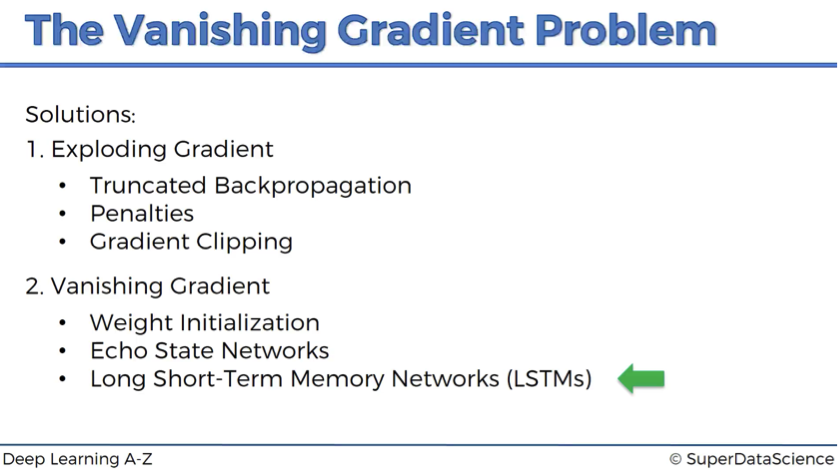
In case of exploding gradient, you can:
- stop backpropagating after a certain point, which is usually not optimal because not all of the weights get updated;
- penalize or artificially reduce gradient;
- put a maximum limit on a gradient.
In case of vanishing gradient, you can:
- initialize weights so that the potential for vanishing gradient is minimized;
- have Echo State Networks that are designed to solve the vanishing gradient problem;
- have Long Short-Term Memory Networks (LSTMs).
LSTMs are considered to be the go-to network for implementing RNNs, and we’re going to discuss this solution in depth in our next article.

Additional Reading
You can definitely reference the original works of the most significant contributors to this topic:
- Untersuchungen zu dynamischen neuronalen Netzen by Sepp (Joseph) Hochreiter (1991). Please note that it is completely in German.
- Learning long-term dependencies with gradient descent is difficult by Yoshua Bengio et al. (1994).
We also recommend looking into the following paper, which is quite recent and by the way, has got Yoshua Bengio as a co-author:
- On the difficulty of training recurrent neural networks by Razvan Pascanu et al. (2013).
That was the vanishing gradient problem. Can’t wait to know the solution to this fundamental problem? Then move on to our next article on the Long Short-Term Memory Networks.

