SDS 771: Gradient Boosting: XGBoost, LightGBM and CatBoost, with Kirill Eremenko

This is episode number 771 with Kirill Eremenko, the founder and CEO of SuperDataScience. Today’s episode is brought to you by Ready Tensor, where innovation meets reproducibility, and by Data Universe, the out-of-this-world data conference.

00:00:20

Welcome to the Super Data Science Podcast, the most listened to podcast in the data science industry. Each week we bring you inspiring people and ideas to help you build a successful career in data science. I’m your host, Jon Krohn. Thanks for joining me today, and now let’s make the complex simple.

00:00:51

Welcome back to the Super Data Science Podcast. Today we’ve got another special episode with our most special of special guests, Mr. Kirill Eremenko. If you don’t already know him, Kirill is founder and CEO of SuperDataScience, an e-learning platform that is the namesake of this very podcast. He founded the Super Data Science Podcast in 2016 and hosted the show until he passed me the reigns a little over three years ago. Kirill has reached more than 2.7 million students through the courses he’s published on Udemy, making him Udemy’s most popular data science instructor of all time.

00:01:26

Today’s episode is a highly technical one focused specifically on Gradient Boosting methods. I expect this episode will be of interest primarily to hands-on practitioners like data scientists, software developers, and machine learning engineers. In this episode, Kirill details decision trees, how decision trees are ensembled into random forests via bootstrap aggregation, how the AdaBoost algorithm form a bridge from random forests to Gradient Boosting, how Gradient Boosting works for both regression and classification tasks. He fills us in on all three of the most popular Gradient Boosting approaches, XGBoost, LightGBM, and CatBoost, as well as when you should choose them. All right, you ready for this extremely illuminating episode? Let’s go.

00:02:14

Kirill, welcome back to the SuperDataScience Podcast. We are all so delighted to have you back yet again for another technical episode this time on Gradient Boosting. You were here back in January for a technical intro to large language models. Then you came back in February to build deeper and dig into encoder decoder transformers, so like a specialized further deep dive. It was volume two of this super popular January episode, one of our most popular episodes ever, and then now you’re back for Gradient Boosting, which is quite different from LLMs, but also super valuable, super powerful. It’s going to be an awesome episode. Thank you for coming on. 

Kirill Eremenko: 00:03:01

Thanks for having me, Jon. Very exciting. Probably I should say that for the benefit of our listeners that even though the space between the episodes is only about a month and a half or so, the knowledge I’ll be sharing today comes from a course that we’ve just released, but we started this course back in end of 2022. Then we put a big pause on it, so it’s not like I just put together something in a month on Gradient Boosting and I’m back here. No, it actually took a few months of research back in 2022 and then finalizing it in the past month to get it to where it is. I’m very excited now to come and share the knowledge we’ve learned creating the course for the benefit of the podcast listeners as well. 

Jon Krohn: 00:03:48

Nice. When you say we, you mean Hadelin right? Hadelin de Ponteves is your co-instructor on the course? 

Kirill Eremenko: 00:03:55

No, it’s just me. 

Jon Krohn: 00:03:57

Oh. 

Kirill Eremenko: 00:03:57

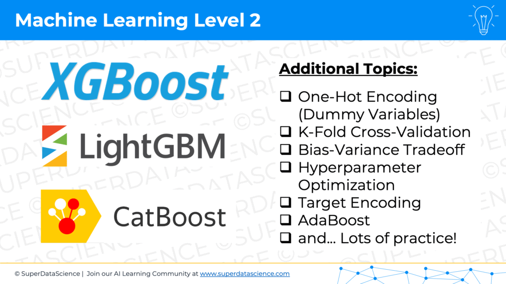
I’m joking. I’m joking, but you know how kings say we? I don’t know, the royal we, yeah, yeah. No, of course. Yes. Hadelin and I, we’ve just published a course. It’s called Machine Learning Level 2 because we have a Machine Learning 1 for complete beginners. Then Machine Learning Level 2 is for practitioners who are intermediate and want to go advanced, and it’s all about Gradient Boosting. The reason for that is Gradient Boosting is, and the underlying techniques, specifically XGBoost, LightGBM, and CatBoost are by far some of the most used and reliably used modeling techniques in industry and in business. 

00:04:39

If you’re not doing deep learning, which is more for mostly, in my understanding is used for new tasks, novel problems, research based things. Of course, it has its applications in industry as well, but if you want just a reliable solution to a classification or aggression problem, XGBoost is one of the… XGBoost, LightGBM, or CatBoost are some of the go-to solutions. We want to equip our students with the best tools to make them successful in their careers. Doing fun stuff in machine learning AI is sometimes different to what you need to get the job done, and Gradient Boosting often is the solution to get the job done. 

Jon Krohn: 00:05:20

Yeah, that reminds me that you and Hadelin were back on the show in episode number 649 for an intro to machine learning to your level one course as well as just a general Machine Learning 101. Yeah, this is now your fourth appearance in just a little over a year. That episode actually also, by the way, was the 10th most popular episode of 2023. We recently- 

Kirill Eremenko: 00:05:46

Oh, yeah, I just listened to your podcast on that today in the car. Yeah, it was funny. I was listening to it. I was like, you mentioned the episode. I didn’t realize you’re going from lowest to highest top 10, and I thought, “Oh, we were number one in 2023, but we were number ten.” 

Jon Krohn: 00:06:01

You barely squeaked into the top 10.

Kirill Eremenko: 00:06:05

I know, I know. Anyway, so yeah, that was about a year ago. That was for Machine Learning Level 1, and now we’ve had lots of people asking for Machine Learning Level 2. We’ve been delaying it because of other projects we’ve been working on, but now we finally released it. It’s just gone live, very excited about, it’s six and a half hour course. Of course, we’ll go into a lot of concepts in this podcast, but right away I wanted to say if somebody wants to check it out, you can find it at www.superdatascience.com/level2. You’ll need to subscribe to SuperDataScience membership. You’ll get access to that course, which is exclusive to SuperDataScience, not available anywhere else. Plus you’ll get access to the Large Language Models A-Z course, which is also exclusive to SuperDataScience, and all of our other 30 plus courses, our community, our workshops at Live Labs that we’re doing twice a month now, career sessions, et cetera. Worth checking it out at www.superdatascience.com/level2. 

Jon Krohn: 00:06:56

I recently organically noticed how many live sessions you’re having in there, very cool. It sounds like the community is really starting to flourish at www.superdatascience.com. That’s cool. I also wanted to add, earlier you were talking about deep learning versus Gradient Boosting or decision trees in general and why you might use one or the other. I think one of the easiest ways, conceptually for me, is that when you are dealing with very large data inputs like an image, or a video, or natural language, that’s where deep learning, including deep learning transformer architectures tends to be very effective. But when you’re dealing with things like tabular data that you could put into a spreadsheet, that’s where the kind of Gradient Boosting that we’re talking about today tends to be the leading approach. 

Kirill Eremenko: 00:07:51

Absolutely. I was actually looking into this yesterday to see the differences, and you’re absolutely right. Deep learning and [inaudible 00:08:04] related things are very powerful when you have additional structure to the data, whether it’s like an image and so on, or you have tabular data with additional structure, you have a time series behind it with some specifics that are not just captured or not easily captured in normal tabular data. If you have ordinary, normal tabular data, which happens to be the most common type of data that businesses aggregate consciously and process these days, whether it’s time sheets or maintenance or medical patient data, whatever, it’s mostly tabular data. 

00:08:42

That’s what you usually find in business and industry without any additional pattern to it that deep learning can catch on and take advantage of. Then you can still apply deep learning, but XGBoost is just going to be Gradient Boosting models is going to be faster, more reliable, easier, quick win, and it’s just a more standard approach to these kinds of problems. You don’t have to reinvent the wheel, just apply it and off you go, some fine-tuning and you’re done. 

Jon Krohn: 00:09:15

Exactamundo, amigo. 

Kirill Eremenko: 00:09:17

Yep. Yep. Okay. Shall we start? We’ve got some exciting topics coming up. 

Jon Krohn: 00:09:22

Yeah, yeah, let’s rock and roll. 

Kirill Eremenko: 00:09:23

Okay, cool. Cool. The first thing we’re going to talk about is ensembling methods in general. What are ensembling methods and how do they work? An ensembling method, first thing that you need is typically ensembling methods they… It’s ensembling methods when you aggregate lots of models to produce one model. It’s like one model that combines lots of models, and there’s two main ways of combining models. But first, before we go to the two main ways of combining models, we need to realize that ensembling methods rely quite heavily on weak learners. They don’t need the individual models that you’re ensembling to be very smart or sophisticated. Typically, it’s something simple. It doesn’t have to be a decision tree, but in most cases, people choose decision trees because they A, are weak learners. B, they’re quick learners, and C, they capture non-linear relationships. 

00:10:25

Having said that, you can use a hundred linear regressions to create an ensemble of linear regressions if your specific use case requires that, but we’re not going to go into custom use cases like that. We’re going to look at the typical approach, and the typical approach is like take decision trees, put them together and get the ensemble. In case somebody needs a quick refresher or somebody’s brand new to this, a refresher on decision trees. Basically just imagine like yes, no splits, right? Yes, if- else conditions. At the start you’ll be like, you have all this data. Let’s say you have a thousand customers and you’re modeling how much future customers will spend on your online store where you’re selling candles, for example. I was thinking, what would we be selling? Candles. I don’t know, some food supplement or something like that.

Jon Krohn: 00:11:20

Yeah, I don’t know. Candles is such a random example. Do you like rooms that smell nice, Kirill? Is that- 

Kirill Eremenko: 00:11:25

I do like rooms that smell nice, but I’ve been recently learning that candles are not regulated. I don’t know about the US, but in Australia, they don’t have standards, so you got to be careful because the stuff they put in might not be healthy for you. 

Jon Krohn: 00:11:37

One in every hundred is actually a stick of dynamite and you don’t know.

Kirill Eremenko: 00:11:42

That’s too funny. Oh, okay. All right. Let’s say you have a thousand customers and you want to predict based on those customers, the new customers are coming into your store in the future, how much they’ll spend in your store. It’s a regression type of problem, and what you will do is you’ll model your existing customers with a decision tree, and let’s say the decision tree splits out the following, the structure. At the top it’ll be a split on let’s say their estimated income. You have a variable of their estimated income, you’ve estimated it somehow, it’s in your input data, and you’re saying… The decision tree will say at the top, the first split is “Is there estimated income less than $47,000 per year or not?” If it’s less than $47,000 go left. That’s a yes. Go, right if it’s a no. In case, and then you just visualize this tree, it’s like a box. It doesn’t look like a tree. It’s like a box. Yes, no, then it’s an if-else condition. If you- 

Jon Krohn: 00:12:41

It’s like an upside down tree. It’s a tree upside down. 

Kirill Eremenko: 00:12:43

Yeah, kind of it grows. Yeah, it grows upside down. That’s right. It’s right. At the top is the beginning of the tree. Is it called the root of the tree? 

Jon Krohn: 00:12:51

Yeah, the root of the tree.

Kirill Eremenko: 00:12:52

Yeah. Okay. The root of the upside down tree. Then you go left if they do earn less than $47,000 per year, then you have another split, so you have another branching of the tree, and then let’s say the condition tree from training has decided that the condition should be, “Is there age less than 45?” If yes, then go down to the left and we’re going to keep it a simple, relatively shallow decision tree, and that’s where we’ll end for that branch, and it’ll be, it’s called a terminal leaf. 

00:13:24

That terminal leaf will have a value. What that value is that during training, out of all of the thousand customers that you have, all of the ones that fell into that branch that had income of less than $47,000 and age less than 45, it’ll take the average. For regression problem, it just takes the average of the customers that they spend there, and let’s say it’s $23. On the other hand, if the customer earns less than $47,000, but their age is not less than 45, so you go left first and then you go right, then the average of those customers was $15. Then let’s go back to the top. If the customer doesn’t earn less than $47,000, so they earn $47,000 or more, then at the very beginning you would’ve gone, right? There, let’s say there could be a terminal leaf right there. It doesn’t have to be symmetric. We’ll talk about symmetric trees further down in this podcast. 

00:14:17

There could be another leaf there. But there, let’s say there’s another split, and it’s asking, “Is that customer signed up to your loyalty program or not?” It’s a categorical variable. If they are signed up, it’s a yes, then you go left down the tree, and because they’re signed up to a loyalty program, their income is over $47,000, the average of those customers that ended up in that bucket is quite high. It’s, let’s say, $212 that they spend on your candles per month or whatever it is that you’re modeling. But if they are not signed up to your loyalty programs, you would’ve gone right in that last branch. Let’s say the answer is there is 48 in the terminal leaf. That’s the average.

00:14:56

You get this decision tree that was built through training, and now any new customer that comes into your company, you can, based on these variables, you can model them and you can see, “Oh, is their income less than $47,000 or not,” go left or right. Then if let’s say they go left, you’re like, “Okay, is their age less than 45 or not?” If their age is 45 or more, then you go, right, and then you know, “Oh, okay, most likely they will spend on my candles in next month $15.” Then you can make business decisions from that. That’s like a simple refresher on how decision trees work. As you can see, it’s quite straightforward and they can capture non-linearity because of these if-else splits. 

Jon Krohn: 00:15:39

Research projects in machine learning and data science are becoming increasingly complex and reproducibility is a major concern. Enter Ready Tensor, a groundbreaking platform developed specifically to meet the needs of AI researchers. With Ready Tensor, you gain more than just scalable computing storage model and data versioning and automated experiment tracking. You also get advanced collaboration tools to share your research conveniently and securely with other researchers and the community. See why top AI researchers are joining Ready Tensor, a platform where research innovation meets reproducibility. Discover more at readytensor.ai, that’s readytensor.ai. 

00:16:20

All right, so to recap back for the audience, this decision tree concept, definitely extremely easy to understand with a visual. 

Kirill Eremenko: 00:16:29

Yeah, for sure.

Jon Krohn: 00:16:30

But it’s the idea, yeah, the base of a tree, which for some reason… I guess because it ends up being on the top of the diagram because we read from top to bottom to bottom, so it makes sense to have the flow be from top to bottom, but that means that the tree shape is upside down. The base of the tree or the root of the tree is the starting point, and you have your first split right at the very top. Typically, I think with most of these approaches… I’m not the expert. I think you’re much more expert than I am, but typically that first split is it is often the most important split. It’s the split that’ll get you your biggest delta in whatever outcome. In your case, is somebody likely to spend a lot of money on candles on my website or not? That first split will often be a variable amongst all the variables available that is going to get the biggest, it’s going to have the biggest relationship. 

Kirill Eremenko: 00:17:21

Yeah.

Jon Krohn: 00:17:22

In this case, in your example, it was income, which makes a lot of sense. People with more income are more likely to spend money on candles on your website. Then from there, you go two ways on this path tree of possible decisions. I guess you can also imagine it like going on a journey. You are walking along a path and the path splits in two, all of the people with high incomes go one way. All the people with low incomes go the other way. Then once you get a little bit further along the path, the people with the high incomes, they encounter another split in the road. This time it’s split on age, and so all the young- 

Kirill Eremenko: 00:18:02

No, sorry, sorry. It’s not a… That’s for the higher earners. For the higher earners, it’s loyalty program. 

Jon Krohn: 00:18:09

Oh, right, right, right. Sorry. Yeah, I messed up. But for the visual analogy, the higher earners, they’re going along their path in the woods and then it splits again a little while later. The ones, the higher earners on the loyalty program go one way. The higher earners that aren’t go the other way and the same thing happens on the other side, but like you said, it doesn’t necessarily need to be symmetric. It doesn’t need to be the same variables that you’re splitting on. The low income earners as they walk along their path, when they encounter a split, they have to split on their age instead of on the loyalty program. Yeah, I’ve never thought of it that way as the path, but I think that’s easy… At least in my head as I’m speaking, it’s quite an easy thing just to imagine that you’re on this journey. 

Kirill Eremenko: 00:18:55

I love it. Yeah. That’s good for visualizing training, exactly how it would happen in training. Then a new candidate that comes onto your website would have to go down this path and look at the signs. I think we should rename decision trees to decision paths going forward. It’s brilliant, seriously. 

Jon Krohn: 00:19:12

When you get to the end, so in this case, so you could have… It’s a hyper parameter in your model when you set it up. You could have lots of levels, lots of bifurcations in the path. It’s always two, by the way. You never get to a point on this journey and there’s three possible paths. It’s always two. 

Kirill Eremenko: 00:19:31

It’s always if-else.

Jon Krohn: 00:19:32

Always if-else, like you said. When you get to the end of that journey, which is a leaf node, so again, if you imagine the terminal node, leaf node, if you imagine- 

Kirill Eremenko: 00:19:42

Leaf node. 

Jon Krohn: 00:19:44

A terminal leaf node, if you imagine that the tree was upside down, these would be a whole bunch of leaves emanating out from the base of the tree. It’s like holding a Christmas tree upside down after you’ve already… It’s Christmas is over and now you’re taking your Christmas tree out of the house. That’s what a decision tree looks like. Yeah, you’re holding it from the base up by your head. When you get to that terminal leaf node on our path analogy, then you could imagine that you’re asked at that terminal point, “How much did you spend on candles at the website?” Then you can average all the people who got to that terminal node. You have different values. Yours, your high income earners who signed up to the loyalty program, they had an average of $212 spent. 

Kirill Eremenko: 00:20:36

That’s right. 

Jon Krohn: 00:20:38

And so on. We might be belaboring what decision trees are now to people who were already familiar with them, but for people who weren’t, hopefully this discussion has been-

Kirill Eremenko: 00:20:49

Hopefully the people who were already familiar with them, forgive us for this slight easy concept detour, because that was important for everybody to get on the same page. From now on, everything’s going to be a lot of fun, and we’re going to dive into more advanced topics. Right away, I wanted to also say that decision trees can be used for regression as we just discussed, and they can be used for reclassification. As you can imagine, reclassification is even easier. You go down these paths, as Jon was saying, during training, customers go. Then there’s a yes, no question, “Did this customer churn or did this customer not churn? Does this patient have cancer? This patient does not have cancer?” Based on what you get through training, your final decision tree will either assign, you can set it up to assign a label. As soon as a new candidate goes through the tree and gets to the end, you can assign a label cancer or no cancer, or in case of classification problems, you can do that, or you can assign a probability if you like, 70%, 20%, whatever else. 

00:21:57

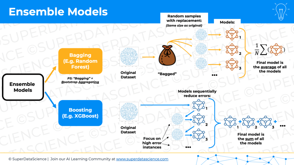
It’s two kind of ways to set it up for classification problems. That was a basic decision tree. Let’s get to the fun stuff, ensemble models. Ensemble models combine weak learners. As we established decision trees are great candidates for weak learners. There’s two main ways of building ensembles. One is called bagging, the other one is called boosting. We’ll start with bagging. Bagging is a cool term because it’s actually short for bootstrap aggregating. It’s just one of those times in life when the real technical term, bootstrap aggregating, actually abbreviates to a cool world bagging, which properly describes the concept.

00:22:35

I was reading about bootstrapping yesterday and really interesting etymology of this word. Bootstrapping comes from some boots, especially cowboy boots, on the back of the boots, they have these straps. I don’t know what they’re for, maybe hanging them up or something like that. You know what they’re for? 

Jon Krohn: 00:22:53

No idea. 

Kirill Eremenko: 00:22:54

Okay, so bootstrapping is kind of like, let’s say you have a fence in front of you and you need to get over the fence and nobody’s around to help you. Well, the idea of bootstrapping is you pick yourself up by these bootstraps and you throw yourself over the fence, something that’s physically impossible. You don’t have… It’s just weird, you can’t pick yourself up. It just doesn’t make sense. But that’s where the term comes from. Visualize that jump, picking yourself up by the bootstraps. In terms of statistics, there’s how it’s applied. Why is it called bootstrap aggregating? 

00:23:26

Well, the whole concept of these bagging type of models, let’s say you have a data set of a thousand observations, and in statistics, you don’t want to… Let’s say you don’t know the underlying distribution of this data set, or you don’t want to make assumptions about this underlying distribution of this data set, and you want to make some inferences from it. What the process of bootstrapping is in statistics is taking this thousand observation dataset and taking samples out of it. You take, just imagine you put all of this thousand dataset, a thousand samples into a bag, and you pick out a thousand with replacement. You pick out a sample, you note it down which one you picked out, you picked out, I don’t know, sample number 747. Then you put it back down, back into the bag, then you pick another sample and so on. 

00:24:15

You pick out a thousand samples, but because you’re doing it with replacement, that means that you might, and you likely will pick out same samples several times and some samples will be missed. That way you’ve just now created, and from your original sample, you’ve created a new sample of a thousand that is different to the original, but it consists of the same total observations. You do that multiple times. You bootstrap, let’s say a hundred times, now you have a hundred samples, and now you can make certain inferences like apply… I don’t know. The central limit theorem to that, or the law of large numbers, things like that, just do statistical inferences from that. Effectively why it’s called bootstrapping is because you’ve done the impossible. You only had one dataset of a thousand samples, and then you’ve lifted yourself up by these bootstraps. Nobody was there to help you. You didn’t make any assumptions about underlying data, and yet you created a hundred samples, which are all different, and now you can make statistical inferences. That’s called bootstrapping.

Jon Krohn: 00:25:16

Kirill, I looked up why boots have bootstraps. It’s pretty obvious, they’re for pulling on the boots.

Kirill Eremenko: 00:25:24

Oh. We’re idiots. Yes, of course. Oh, I love it. Yeah, that’s good. Yeah, to help you put them on. Yeah, was my description of bootstrapping, correct for statistics? 

Jon Krohn: 00:25:37

Oh, it was unbelievable. I feel like there’s almost even no point in me saying it back to you in my own words because it was beautiful. 

Kirill Eremenko: 00:25:43

Awesome. Thank you. 

Jon Krohn: 00:25:44

Bootstrap aggregation. Yeah, picking yourself up by your own bootstraps. That’s a common expression. I think it’s been around for a very long time. But yeah, just this idea that you’re without, you’re not really simulating new data. You’re not simulating new individual samples. You’re not needing to go out and collect new data. You are bootstrapping based on what you have, and you’re creating a whole bunch of samples with just what you have, so it’s bootstrapping.

Kirill Eremenko: 00:26:10

That’s right. Bootstrap aggregation is the process of bootstrapping many times and then doing some analysis and aggregating. In the case of ensemble methods, that’s exactly what we’re going to be talking about. We’re going to be doing bootstrap aggregating as we can see just now. But I just wanted to make a quick comment that the term bagging, like the abbreviation bagging, makes perfect sense because you’re putting these samples into the bag and then you’re pulling them out of the bag. It’s a good mnemonic to remember what bootstrap aggregating is. 

00:26:42

Let’s talk about ensemble methods. We are already into this first one called bootstrap bagging, short for bootstrap aggregating. Let’s talk about an example of a bagging method. That one to many of the listeners will be familiar. It’s called random forest. What you basically do with random forest is you do bootstrap aggregating. You’d say you have a thousand samples. You want to create a random forest, which is an ensemble method, combining decision trees. Let’s say you want to have a hundred decision trees in this random forest. You do bootstrap aggregating. You create a hundred different samples based, each one has a thousand observations based on your original one, just the way we just described, using that bootstrapping method. Then you build a decision tree from each one of these samples. Each one of the decision trees will see a slightly altered version of the original data.

00:27:34

Therefore, each one of these decision trees, even though they might have the same, they will have the same hyper parameters. Their tree structure and the breaks and the splits in the tree will be different. Then you get the results of each decision tree and that the final model, the random forest prediction, will be the average for… Basically will be the average of these decision trees. Let’s say you’re talking about this candle sales example and how much each customer will spend. Instead of building one decision tree and predicting based on that, what you can do is do this bootstrapping process, build a hundred decision trees, each one with slightly different underlying data. Then see, let’s say for a new customer that comes through into your store, you see what each model will predict. 

00:28:26

Some models will predict $23, some models will predict $15, some $212, et cetera, et cetera, et cetera, or other values because each tree is built differently. Some models might predict $78. Some models predict $300 depending on how the tree was built. Then you’ll just take the average. You’ll say, “Okay, so this customer came into the shop.” These hundred decision trees make their predictions. The average of what the random forest predicts is $51 and 23 cents. That will be your final output from the random forest. That’s what you’re going to use.

Jon Krohn: 00:29:03

This episode is brought to you by Data Universe coming to New York’s North Javits Center on April 10th and 11th. I myself will be at Data Universe providing a hands-on generative AI tutorial. But the conference has something for everyone. Data Universe brings it all together, helping you find clarity in the chaos of today’s data and AI revolution. Uncover the leading strategies for AI transformation and the cutting edge technologies, reshaping business and society today, data professionals, business people, and ecosystem partners, regardless of where you’re at in your journey, there’s outstanding content and connections you won’t want to miss out on at Data Universe. Learn more at datauniverse2024.com. 

00:29:42

Yeah, random forests are amazing, powerful models. What you’re going to get into next with Gradient Boosting, it makes them even more powerful, but random forests on their own, they make that decision tree idea that we walked through in detail. The idea of going down those paths, or the upside down Christmas tree, when you only have one of those upside down Christmas trees, it’s relatively… 

Kirill Eremenko: 00:30:04

Terrible. 

Jon Krohn: 00:30:04

Limited, yeah. The advantage of that kind of single decision tree is that it’s very easy to understand. You can see it, you can see each of the bifurcations in the path, and you have very clear end values. But with a random forest, when you bootstrap aggregate a whole bunch of different samples, and then maybe randomly turn off some of the input variables for some of those random forests optionally, you end up with a super powerful machine learning model already. Random forests are amazing. They’ll often get you near the top possible performance on tabular datasets, like we talked about at the beginning of this episode already. Random forests are super powerful, but the boosting now that we’re going to get into, that you’re going to get into, is even more powerful. Where random forests fall down, boosting managed to fill in the gaps, and do even better. 

Kirill Eremenko: 00:31:04

Yeah, absolutely. Before we get to boosting, I wanted to give a real-world analogy for random forests that really helped me understand this concept. Have you ever been to a fair, Jon? 

Jon Krohn: 00:31:17

Sure, yeah. 

Kirill Eremenko: 00:31:19

You go to a fair and there’s rides, and roller coasters, and other little games that you play, and so on. One of the games that you sometimes see at the fair is this big jar with lots of jelly beans inside, thousands, and you need to guess what the number of jelly beans is in there. You’ve seen that one? 

Jon Krohn: 00:31:37

I’ve seen that one. When I was a kid, actually, it wasn’t at a fair, but it was at a friend’s house. It was his birthday party, and there were 20 kids, and they had this game. I might’ve been maybe 10 years old, and I guessed the number of jelly beans on the dot. 

Kirill Eremenko: 00:31:50

Wow, very good. Very good. Basically, the principle is the person who gets closest wins the prize, or maybe some rules might be different, but let’s say you might have to guess on the dot, like Jon did, or the person who guesses closest, or within a certain range. 

Jon Krohn: 00:32:11

You just have to get closest, I think. 

Kirill Eremenko: 00:32:14

What the most optimal strategy for this is, you combine a ensemble of weak learners, and because humans are not designed to predict the number of jelly beans inside a jar, where there’s thousands of them, or hundreds- 

Jon Krohn: 00:32:31

Speak for yourself. 

Kirill Eremenko: 00:32:33

You seem to be very good at it. Humans, apart from Jon, are not designed for doing this. 

Jon Krohn: 00:32:38

I’m batting one for one on jelly bean guessing. I’m never going to do it again.

Kirill Eremenko: 00:32:43

Keep it high. Keep your stats high. Humans are bad at that. Humans are perfect weak learners. What you need to do is, you get a notepad and a pen, and every time somebody comes to the stand and makes a guess to whoever owns this challenge, when they walk away, you ask them, “Hey, what was your guess?” You just write it down, and then the next person comes and guesses, the owner or whatever tells them if they’re close or not. Doesn’t even tell them, just writes it down, writes the contact detail, to contact them if they’re a winner. Then they walk away, and they walk past you, and you ask them again, “What did you guess?” You ask everybody who made a guess what they guessed. 

00:33:22

Unless there’s some sort of trickery going on, like it’s a hollow in the middle type of jar or something like that, if there’s no trickery going on, you’ll get hundreds of these guesses which are a bit high, a bit low, a bit high, a bit low, and so on and so on. But then you take the average of them, like a random forest does, you created a own ensemble. You take the average, and the average will be the best guess. The average, in many cases, will be the closest to the actual amount, because people have their own differences in their thinking, in their perception and so on. Some will guess higher, some will guess lower, but on average, you’ll be very close. If, the next time you’re at a fair, you see one of those, give that a try. In general, in my view, that’s a great analogy of what a random forest does. 

Jon Krohn: 00:34:06

That was a really nice analogy. Another one that is worth mentioning quickly is just that visual of this random forest. The clue of what’s happening there is right in the name. You take a whole bunch of decision trees, and trees make up a forest. Each of those trees in the forest is slightly random, a random forest, in that there are different bootstrap aggregated data sets that make up each of the individual trees, so there’s randomness there. As I mentioned earlier, there’s also randomness around, sometimes optionally, what input variables are being considered, what independent variables are being considered. 

Kirill Eremenko: 00:34:47

Yes, the features. 

Jon Krohn: 00:34:48

The features, yeah. 

Kirill Eremenko: 00:34:49

The feature selection. There’s selection by bootstrapping, the underlying rows are different. But also, you could set a parameter saying that, “The trees don’t see all of the features, they only see 80% of the features randomly.” Each tree not only sees different rows to other trees, but also sees different columns, and that’s a great way of combating over-fitting.

 

Jon Krohn: 00:35:15

Going back to your earlier example of the single decision tree, where three of the variables that you got into were income, age, and whether they were signed up to the loyalty program or not, in a random forest, the first tree in the random forest might only have income and age. Then randomly, the second tree has age and loyalty program, and so on. You get slightly different answers every time. 

Kirill Eremenko: 00:35:43

Yeah, and it’s actually a good point to say that trees can reuse variables. If it used income at the top and then it used loyalty program in the next split, and again, can use income. It is not limited to using a feature only once. It can be done as well. There’s other hyperparameters, like the depth of the tree. You could set the maximum depth to eight or whatever. There’s a hyperparameter for a random forest. You can set how main trees, 100, 1,000, how many trees you want, et cetera. We’ll get a bit into that further down. I feel it’s important to also mention quickly, on random forests, you can also use it for classifications. What we just discussed was regression.

00:36:20

Just keep in mind, throughout this podcast, we’ll be talking about regression classification from time to time. Those are two big separate types of problems that are solved with all the methods, what we’re discussing. You can also use it for classification. A random forest for classification would be, rather than taking the average of all of the trees that you have, you would use it as a voting system. It’s like a democracy, a democracy of random trees. Basically, the trees make their predictions, will this customer churn? Will this customer not churn? For a medical data set, does this patient have cancer or not? 

00:36:53

Then you have these predictions from all the trees. Basically, you look at it like a vote. Out of 172 trees voted that this customer does not have cancer, 28 voted that they do have cancer. You could say that’s a no, or if you want to be more cautious to avoid what is going to be a type two type of error, where you’re saying they don’t have cancer but they actually do, you might say, your threshold is not 50/50, your threshold is 75/25. In this case you’ll say, yes, they have cancer, just to make sure and double check. Basically, you’d use it as a voting system. 

Jon Krohn: 00:37:30

Yep. 

Kirill Eremenko: 00:37:30

Cool. All right, let’s move on to boosting, so excited. All of that was up to… which year was that? Up to 1995, and 1995 was the first year when boosting was introduced conceptually. It didn’t become very popular as this random forest until around 2016, when XGBoost came out, and we’ll get to that further down. 2014, that’s when XGBoost came out. Random forest was dominating, and for example, Kaggle competitions, a lot of people were using random forest all the way up to 2014, 2015. Whereas boosting slowly started growing, got developed and started growing from 1995. 1995 was when two authors, Yoav Freund and Robert E. Schapire, I’m not sure if I’m pronouncing that correct, Schapire, from AT&T Labs, they published a paper. Actually, no, they didn’t publish a paper. They developed the concept of Gradient Boosting and then later, they published their paper in 1999. Sorry, not Gradient Boosting, they didn’t develop Gradient Boosting. They developed the concept of AdaBoost, so just boosting. The method, the model that we’re going to talk about is called AdaBoost. Just keep in mind, very important, AdaBoost is not a Gradient Boosting model. 

Jon Krohn: 00:38:53

The Ada there stands for adaptive.

Kirill Eremenko: 00:38:55

Exactly. Thanks Jon. It’s adaptive boosting. They got the prestigious Gödel Prize in 2003 for their work. It is for theoretical computer science. It’s like the Nobel Prize, I guess, or a Nobel… actually, Gödel himself got the Einstein Prize. A Gödel Prize is a prize, but it’s tiny. For somebody in this space, it wouldn’t be a lot of money. I believe it’s $5,000, so it’s not a huge amount of money, but at the same time, it’s more prestige. They got this prize in 2003.

00:39:29

Okay, let’s talk about AdaBoost and how it works. AdaBoost was the first boosting method, and their thinking was, “All right, why are we doing these random forests? Why don’t we adjust the approach?” In AdaBoost, what you do is, you take your 1,000 samples from your candle store, and you’re going to train an ensemble, again, of weak learners. They’re going to be decision trees. First decision tree, you train it on the full sample that you have. No bootstrapping, you just train it on the 1,000 people that you have, 1,000 observations that you have. Then you look at, how well did this model perform? On which observations did it do well? On which ones did it not do well? Some observations, the errors will be low. On some observations, the errors will be high.

00:40:26

What you do is, you take the observations that had high errors, and you assign them a weight, a higher weight. The lower the error, the lower the weight, the higher the error, the higher the weight. Now, you start doing bootstrapping with the same data set. You take the 1,000 samples, you put them in a bag, you’re going to pull out of the bag with replacement, so bootstrapping, but the way this bag is created is, the observations that had higher errors will have higher weights in this bag. This is a very simplified explanation. We’re not going to go into too much detail in this, but just think about it like you have this bootstrapping method, but the observations that initially, in the first prediction had higher errors, they’ll have a higher chance of getting picked out of the back. 

00:41:11

Now, you bootstrap this new data set, or again, 1,000 observations, but it’s geared towards the observations that you didn’t predict that well in the first instance. Now, you make a second decision tree to predict the results for this new bootstrap data set, and again, you get some of them that you predicted well, some of them that you predicted not so well. Again, you assign weights based on that. Now, you take the original 1,000 and you create another bootstrap, but you apply those weights that you had just assigned from the second result, and so on.

00:41:49

Every time you’re bootstrapping, you are adjusting to favor the observations that you didn’t predict well in the previous iteration. You keep doing that. Let’s say you have 100 decision trees, so you do that every time. In addition to that, you also look at how well each decision tree performed overall. Each decision tree, you assign it a score based on how well it predicted overall. What’s its overall error? Then in the end, you will have 100 decision trees. Each one is focused on predicting better the samples that were miss… by the way, AdaBoost was originally developed for classification, so it’ll focus on classifying better the samples that were misclassified by the previous decision tree, and that is done through the weighted bootstrapping process. Also, each one of the decision trees will have a score based on how well it performed overall in its job.

00:42:48

The final model results, rather than like in a random forest, where we took the average of all of these values, or in the case of a classification, we took the votes of all of these trees, in the case of AdaBoost, you take a weighted vote, in this case, it’d be a weighted average, you take a weighted average of all these… you can call it a weighted vote, it’s a plus one/minus one type of thing for classification. You take a weighted average of all of these trees, and the weights are those scores that we assign to each one. Two things are happening. Each model is favoring the observations that were misclassified in the previous model. We are focusing on the errors. The breakthrough in AdaBoost was, let’s not just do random trees, but let’s improve iteratively every time, to focus on the things we didn’t do well in the previous tree.

00:43:40

The second thing is, let’s also consider how well each one of the trees is performing in our final result. Don’t give everybody the same. It’s not a democracy anymore. What is it called? A meritocracy. How well you perform gives you a certain weight. Those were the two, I would say main breakthroughs on AdaBoost. Of course, there’s more to it, but that took it to a new level. It’s no longer just a random bagging, or bootstrap aggregating, it’s conscious. Let’s think of what we’re doing, and iteratively improve on this sequence.

Jon Krohn: 00:44:18

Starting on Wednesday, April 4th, I’ll be offering my Machine Learning Foundations curriculum live online via a series of 14 training sessions within the O’Reilly platform. Linear Algebra, Calculus, Probability, Statistics and Computer Science will all be covered. The curriculum provides all the foundational mathematical knowledge you need to understand contemporary machine learning applications, including deep learning, LLMs and A.I. in general. The first three sessions are available for registration now, we’ve got the links in the show notes for you and these three sessions will cover all of the essential Linear Algebra you need for ML. Linear Algebra Level 1 will be on April 4th, Level 2 will be on April 17th, and Level 3 will be on May 8th. If you don’t already have access to O’Reilly, you can get a free 30-day trial via our special code, which is also in the show notes.

00:45:04

That’s the one line main difference between Gradient Boosting and AdaBoost? 

Kirill Eremenko: 00:45:11

Sorry, no, we haven’t gone into Gradient Boosting yet. The one line main difference between bagging, bootstrap aggregating, which is random forest, and boosting, which is AdaBoost, is the word adaptive, adaptive boosting.

Jon Krohn: 00:45:26

Right. 

Kirill Eremenko: 00:45:26

You’re adapting to boost the observations that you didn’t predict well, that’s what you’re adapting. 

Jon Krohn: 00:45:34

Right. 

Kirill Eremenko: 00:45:34

It’s a conscious method. Rather than, all right, let’s rely on the law of large numbers, and get lots of votes or predictions, and average them out, like a democracy, in AdaBoost, it’s a meritocracy. It’s a conscious meritocracy. Let’s adapt to consciously work on our mistakes, and then also, let’s give not just an average, but a weighted average, because those are not performing well. Why would we consider them in our final average as highly as the ones that are performing well? 

Jon Krohn: 00:46:08

Nice. I actually didn’t know about AdaBoost before, so great to hear about it. Thank you.

Kirill Eremenko: 00:46:14

Yeah, it’s not that popular these days, because Gradient Boosting blows even AdaBoost out of the water, but it was an important stepping stone. I like the history of how things developed. I thought I would mention it, and also, for people’s general understanding. For example, in the course that I mentioned, which you can get at www.superdatascience.com/level2, the number two, we don’t talk much about AdaBoost, but we go into some detail on it. I think it’s good to know the history of where things come from, and if it comes up in a conversation, you’ll know. 

Jon Krohn: 00:46:49

Sure. 

Kirill Eremenko: 00:46:51

Now, we can move on to Gradient Boosting. We’ve laid the foundation. The difference between just bagging, or bootstrap aggregating, a blind democracy, nothing wrong about that, versus a conscious meritocracy, so to speak. Now, we can move on to Gradient Boosting. Gradient boosting was originally proposed by Jerome H. Friedman in 1999, and there’s two papers you can find online. One is called Greedy Function Approximation: A Gradient Boosting Machine, and I think that was more of a lecture that he gave, because it’s got 40 pages or something like that. The second paper you can find is Stochastic Gradient Boosting. This is the person who created it. What is Gradient Boosting, and how is it different to bagging, bootstrap aggregating, and AdaBoost? 

00:47:45

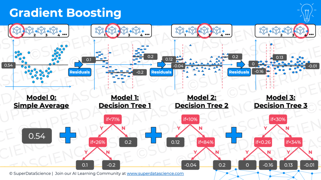
The main thing with Gradient Boosting is that this time, we’re not just going to adapt. We’re going to actually be changing our sample. We’re not going to be doing any bootstrapping. We are working with the original sample all the time. That’s very important to understand. There’s no bootstrapping in Gradient Boosting. What you do in Gradient Boosting is, we’re going to look at Gradient Boosting for regression first. You have your 1,000 customers. I can’t believe this example stuck. That was just a random thing I wanted to do for the trees. 

00:48:19

You have these customers, 1,000 customers that bought candles from your store. You want to predict the future spend of customers. Your target variable is your dollars spent. What you do is, you take as your first step… again, Gradient Boosting is again going to be an ensemble of models. Your very first model is just an average. It’s a simple average. You take the average of all of the dollars that all of your customers spend, and let’s say you get something like $57 for simplicity’s sake. That’s the average of all your customers’ spend. Next, what you do is you calculate the errors. You look at, “Okay, $57 is my average,” that is, of course, a terrible prediction, a terrible model. You just took an average. For some observations, you’ll have an error, some observations will be lower, some observations will be higher.

00:49:14

You basically calculate the error for each one of your 1,000 samples, and then you take those errors, whether the error is $2 or $20 or minus $100, you take all of those errors and you build a decision tree to predict those errors. The first model, it takes the average, works with a sample. The second model, which is our first decision tree, it’ll work with all of the errors that you got as a result of the first model. Now, this decision tree will be structured in some sort of way. It’ll make its own predictions, and now you will have, again, errors. 

00:49:55

You will have errors of this decision tree’s prediction, and some might have $5 error, some might have a minus $50, minus $100. Again, you look at all the errors of the predictions of this second model, which is a decision tree, and you use those errors. Again, you’ll have 1,000 errors, in some cases it might be zero, but you’ll have 1,000 values, and you use those errors, and you make another decision tree. Your third model will also be a decision tree, and it’ll predict the errors of the second model. Then you build a fourth decision tree, which will be predicting the errors of the third model. Then you build a fifth model, which is also decision tree, and you predict the errors of the previous model, and so on. You chain them together. The key word here is, you’re chaining models after each other.

00:50:44

The first one is an average, and then it’s decision tree, decision tree, up to 100 times, however many decision trees you want. Each one is just focusing on predicting the errors. What’s the point of that? Well, guess what? Now, as our final model, we’re not going to take the average, we’re not going to take the weighted average. As the final model, we’ll take the sum. You’ll take your first model, which is the average. You’ll add the result of the second model, which is whatever the decision tree predicts for this kind of variable. Let’s say you have a new customer come into your store, and you want to predict how much they will spend. The answer will be the average, which was $57, plus whatever the next model, model number two, which is a decision tree, whatever it predicts, plus whatever the next decision tree predicts, plus whatever the next decision tree predicts and so on. 

00:51:32

You add all of that up, and because each time you are predicting the errors, now, your prediction is the average plus, what would the error be for this person that just came in? Okay, the error for this person is 57? Okay, based on their age, based on the income, whatever the decision tree is looking at, the error of this second of this initial model would’ve been minus $101. You need to add that. You go from 57 minus 101, I’m not that great. What is it, minus 44? Is that minus 44? Yeah, minus 44. Then the next model will be, what would the error have been based of that prediction, the previous one? The error would’ve been $50. Now you go up to $3, and then the next model says, the error at this point is about $27. 

00:52:25

Now you go up to from $3 to $30, and so on and so on and so on. Then the final result is, this customer, based on their features and based on what the model predicts for them, this customer will likely spend $39 in our store. That’s how Gradient Boosting works. You’re basically chaining models to constantly just predict the errors of the previous one, and that means in the resulting model, you need to just add them up. Each prediction will be a prediction of the errors, and in the end, you will get your final result.

Jon Krohn: 00:53:01

Nice, very well explained. 

Kirill Eremenko: 00:53:04

I just had this idea, it’s probably good to call the first model, the average, call it model zero, because otherwise, it’s confusing. The first decision tree is the second model. The second decision tree is the third model. Model zero is your average, and then model one is a decision tree. Model two is your second decision tree, and so on and so on and so on. The final result is the sum of this chain. 

00:53:29

As you can see, it’s very different to what we had previously, in the bootstrap aggregating methods, which were bagging, basically a random forest, the way we took the average. It’s also different to the boosting method of AdaBoost, where we took a weighted average of the models. AdaBoost is in between. It’s used as bootstrap and it’s used as aggregating, so it’s a bootstrap aggregating method from the sense of how the samples are built, but it’s a boosting method based on the concept. AdaBoost is a transitional, whereas Gradient Boosting is pure Gradient Boosting. There’s no more bootstrapping. Straight into, use the same data set all the time, but you focus on improving, improving, improving, improving. 

Jon Krohn: 00:54:15

To summarize back, the random forest is random. This went into your democracy versus meritocracy example. With a random forest, you are randomly creating a whole bunch of decision trees, and the more that you create, you get this slight marginal improvement. When you go from 1,000 random decision trees to 1,001, there’s this very marginal improvement. The core idea with adaptive boosting was to not be randomly creating these decision trees, but to use some information, like which data points were misclassified previously, and let’s overweight those in the subsequent model so that we’re consciously iterating in the right direction adaptively, AdaBoosting. Gradient boosting takes us another level further by not just saying, “Let’s focus on the data points that were misclassified. Let’s look at the residuals, the specific delta between what the correct answer would’ve been and what the model predicted, and let’s fix those residuals.” You’re focusing on where the most possible opportunity for improvement is, and that’s why Gradient Boosting is so powerful. 

Kirill Eremenko: 00:55:38

Yep, absolutely. Great summary. A question that you, our listener, might have at this stage is, if you’re focusing on residuals, why is it called Gradient Boosting? Why isn’t it called residual boosting, or error correction or something like that? Well, we’ll answer this question right now. The answer lies in the mathematical principles underpinning this algorithm. I’m going to be a bit more out of my depth, a little bit less experienced than Jon talking about this, so Jon, please feel free to correct me if you feel that something needs correcting. Basically, what happens is, the explanation we just looked at, where you look at the residuals and you build every next model in the chain to predict the residuals of the previous one, is correct, but it’s a simplified explanation. The actual underlying mathematics of it is that you don’t look at the residuals of the model. 

00:56:38

This is how it works in proper mathematical principles, Gradient Boosting. Gradient boosting, take two. First thing you do is, you define a loss function. You choose what loss function you’re going to use for this model. Then you will calculate the gradient of the loss function after each model is built. You have your first average, you have your loss function, then, for every one of those 1,000 points, you will calculate the gradient of the loss function, and you will use the next model in your chain. We agreed that the original model is model zero with the average. You’ve done the average, you’ve calculated the gradient of the loss function. By the way, if somebody needs a quick refresher on what a gradient is, a gradient is basically a vector of partial derivatives of the loss function. 

00:57:28

You have a loss function, let’s say it’s based on two variables, X and Y, then the gradient will be a partial derivative of that loss function based on the variable X. That’s your first coordinate in the vector, and your second coordinate is a partial derivative of the loss function based on the variable Y. If you have five independent variables, or five variables in your loss function, then it’ll have five coordinates in the vector. That’s very brief overview of what a gradient is. There is a cool video from Khan Academy, if anybody wants to get a refresher on what a gradient is. Really short, succinct, and gets to the point. Back to Gradient Boosting. You have model zero, which is the average. That’s your prediction. Then you calculate the gradient of your loss function for every single one of those 1,000 points. Your next model, model number one, decision tree number one, is going to be built to predict those gradients that you’ve just calculated. After model one is built, you will calculate the gradient of the loss function for this model number one in every single one of your 1,000 points. 

00:58:43

Now, model number two, decision tree number two is going to be built to predict the gradients that you’ve just calculated of model number one, and so on and so on and so on. That’s why it’s called Gradient Boosting. A gradient, it tells you in which direction your loss function is increasing the maximum, and the higher the gradient, the higher… sorry, it tells you in which direction the loss function is increasing from this point, and the higher the gradient means the higher increase in this loss function. Your point is to minimize your loss function, and by predicting the gradients, that’s what you’re effectively doing, by chaining these models together. 

00:59:22

Now, how does this reconcile with what we just discussed with the residuals? Well, it just so happens that this loss function for regression problems is chosen in a very conscious and deliberate way, and it’s usually the simple squared loss function that is used. Basically, if you think of the mean squared error loss function, which is used for, for example, linear regression, let’s say it’s observed minus predicted squared, the sum of that, and for all the observations, divided by N, number of observations, that’s an aggregate loss function. If you think of it for an individual observation, what is the loss function for an individual observation when you’re using mean squares error? 

01:00:06

Well, the individual observation’s loss function is just observed minus predicted squared. That’s the loss function for individual operation. In the case of Gradient Boosting, we’re using the same loss function, it’s called the simple square loss function, but we are just adding a coefficient at the start, which is one half. The loss function equals, for an individual observation, is one half of brackets observed value minus predicted value, and those brackets squared. When you take the gradient, or you take the derivative of that, the two, the differential of X squared is 2X, so the two comes out and it gets canceled out with the one half coefficient that you have at the beginning. It becomes observed. So the derivative of the loss function is basically observed minus predicted, which equals to the residual. So the loss function is chosen consciously and deliberately in such a way that the derivative of the loss function, which we’re aiming to minimize with this whole method, that derivative of the loss function is the same as the residuals. And that’s where the actual mathematical explanation that we just went through reconciles with the simplified explanation we had earlier about the residuals. And I think that’s really beautiful.

Jon Krohn: 01:01:21

Nice, Kirill. All right, so that was all about regression. What’s different in Gradient Boosting when we have a classification problem? 

Kirill Eremenko: 01:01:29

Okay, so for classification, Gradient Boosting is not as straightforward, is not as simple. The reason for that is, when we chain these models, we can’t just think of it as adding up each… We’d still be adding up models, but you can’t just think of it as simply as we did in the case of predicting the residuals, because in the case of classification, we’re predicting probabilities. And if you start adding up probabilities from 100 decision trees, you’ll end up with probabilities of over one. And basically, it’s not as elegant.

01:02:02

The underlying core principles, so we’re not going to go into detail on that. Again, check out the course if you’d like to learn more, but we’re not going to go into detail on that. The main thing to take away about boosting or Gradient Boosting for classification is that the underlying concept is the same. You calculate the gradients, you define a loss function, and in the case of classification, what is normally used is called a binomial deviance loss function. You calculate the gradient of your… well, the first, the zero model, the model number zero is usually set, it’s not at the average, it’s usually set at 50%. So if you’re, let’s say, classifying between two categories, will churn, will not churn, has cancer, has not cancer, you set at 50%.

01:02:41

Sometimes if you’re more advanced and you have reasons, you can set the baseline at higher, 75% or 25% or whatever else, but that’s up to your specific use case. So you set a baseline in the zeroth model, the original prediction is 50%, whatever you choose. And then basically you have a loss function. You will need to find the gradients of the loss function for every one of your observations, and then the next decision tree will be minimizing that loss function. And when you choose the binomial deviance loss function, which is, as I understand, typically used for classification problems in Gradient Boosting, what will happen is when you’re getting to the gradients, when you’re calculating the gradients, rather than probabilities, you will end up working with log odds. So it’s a very interesting transition, and in the course we explored, it looks really cool.

01:03:41

So you want to predict probabilities, but what the decision trees are actually doing, what the chain of decision trees is doing, is it’s predicting log odds, and that allows you to add them up. So you have the same principle. You will be adding up the predictions of each decision tree, but you won’t be getting probabilities, you’ll be getting a log odds. We’re not going to go into detail what log odds are right now, they’re related to probabilities. And once you add up all the log odds from your decision trees for your prediction, then you go from the world of log odds, you do an inverse operation, and you go back into the world of probabilities, and then you’ll get your final probability.

01:04:20

So that’s just a quick teaser for what classification looks like in Gradient Boosting. Again, if you want to dive into detail, check out the course that we have, Machine Learning Level 2 at SuperDataScience, or feel free to do this research on your own. But yeah, basically the takeaway is underlying concept of gradients is the same, and it works as well for classification as it does for regression. 

Jon Krohn: 01:04:47

Nice. Yeah, as you started to introduce the classification variant of Gradient Boosting, you said it’s not as simple, but actually it wasn’t that much more complicated either. You’re using log odds, you just got to add that in. 

Kirill Eremenko: 01:05:01

Man, log odds. For me, it took a while to get my head around log odds. You’re probably right, it’s not that complex, but it’s just harder to visualize. I like the regression alternative because you’re visualizing this chain, you’re adding up, it makes sense. You’re predicting errors, you’re constantly reducing this error through your prediction. Whereas this one is like log odds, you have to go back to probability. It’s not as easy to just have a picture in your head. 

Jon Krohn: 01:05:26

Yeah. Yeah, yeah, yeah. Nice. All right, so I think then you’ve now gotten through all of the Gradient Boosting, the “vanilla.” Everything that you said so far sounds super amazing, but now I’m adding this vanilla adjective, because it turns out today there’s been several variants on the regular vanilla Gradient Boosting that you’ve described to get even more powerful results, I think. Things like XGBoost, LightGBM, CatBoost. You want to dig into those? 

Kirill Eremenko: 01:05:58

Yeah. Okay, let’s do it. So all of that was foundational and very important. However, up until 2014, Gradient Boosting, again, I’m not an expert or researcher, or historian for that matter, but my impression is that Gradient Boosting was purely or mostly theoretical. It wasn’t very applied, very applicable, because it was slow. Because when you’re building these hundreds of decision trees, you have to find the splits. 

01:06:28

Imagine you have, for example, for salary, you have 1,000 estimated salary. So with only to have just 1,000 people in your sample, you need to make that split. How does the decision tree, one of the decision trees, how does it know that it needs to split at 47,000 more or 47,000 less? Why is it not 46,500? Why is it not 93,000? Why is it not 12,000 or $12,534? How does the decision tree know? And if you have 1,000 samples, of course there’s optimization techniques built in, but it has to look through a lot of options to find out where is that best split, which split is going to give me the best result? Because it only can choose one. At each ranch, it can only choose one split. Even if you have just three variables, it has to look through three variables and through all possible splits inside these variables. So theoretically it’s a cool algorithm, but unless you find ways to speed it up, it’s just going to stay theoretical and you’re going to get bogged down. It’s very slow. And that’s exactly what happened in 2014. A gentleman named Tianqi Chen, I hope we’re pronouncing that right, as part of the… What is it called? OD- 

Jon Krohn: 01:07:55

You’re basically guaranteed to not be pronouncing that right, because you’re not going to know how to do the tones. But I guess- 

Kirill Eremenko: 01:08:00

Yeah. Yeah.

Jon Krohn: 01:08:01

… yeah. Tianqi Chen is a good guess for us people that can’t hear tones. Unless, can you hear? Chinese tones, is that something that you’ve studied?

Kirill Eremenko: 01:08:11

No. No, I have no idea. So I apologize if I mispronounced that. I’m doing my best. I was just looking up the abbreviation for XGBoost. So XGBoost was originally introduced in 2014 as part of this community called DMLC, I think it’s on GitHub, called Deep Machine Learning Community. It was produced by this gentleman, Tianqi Chen, who I believe was a student at the time maybe, or he’s a professor right now. I’m not sure which university. I would guess Carnegie Mellon. I’m not sure. But basically he produced this as part of this open source community in 2014. And the whole principle of XGBoost, the XG stands for eXtreme Gradient Boosting. So the whole principle, as I understand, was to come up with ways to speed it up so we can actually use it in applications and not leave it as a theoretical algorithm for the rest of time. Yeah, go ahead. 

Jon Krohn: 01:09:19

Yeah, you remembered correctly, your instinct was right. Tianqi is an assistant professor at Carnegie Mellon, though it seems like they’re also a co-founder and chief technologist at something called OctoML. So they’re one of those amazing people who’s bridging academia and practical data science. OctoAI is running, tuning, and scaling the models that power AI applications. 

Kirill Eremenko: 01:09:44

We should have them on the show, Jon. 

Jon Krohn: 01:09:45

Yeah, it’s a great idea, for sure. 

Kirill Eremenko: 01:09:47

Sounds like my big [inaudible 01:09:48].

Jon Krohn: 01:09:49

That is certainly the kind of guest I love. We’ve had quite a few guests, yeah, where they do both of those things. Where they’re academics, right on the cutting edge of developing machine learning, but then simultaneously they’re at the cutting edge commercially. That is one of my favorite guests. You’re exactly right. 

Kirill Eremenko: 01:10:08

Yeah. If anyone listening knows Tianqi Chen, author of XGBoost, please shoot him an email and introduce him to the podcast. We’d love to talk to him about it. That’d be cool. Anyway, we are digressing. So after the method came out in 2015, it became very popular. There was a follow-up research paper from Tianqi Chen, which you can find on archive. It’s called XGBoost: A Scalable Tree Boosting System. That was published in 2016. 

01:10:40

Okay, so after the method came out, it became super popular. For example, in 2015, the year after it came out, out of the 29 winning solutions on Kaggle, 17 of them used XGBoost. I think eight of them were pure XGBoost, and nine of them were a combination of XGBoost and deep learning. But nonetheless, 17 out of 29, more than half of the winning solutions in Kaggle, literally the year after, were already using XGBoost. That’s how popular it was. 

01:11:11

Also, on the KDNuggets Cup in 2015, again, the next year, XGBoost was used by every winning team in the top 10. How cool is that? And that’s because, again, I’m not a researcher, but as I understand, XGBoost was the transition from theoretical Gradient Boosting, which sounds amazing but it’s very difficult to apply because of its computational inefficiency and demand for resources and other things, it was the bridge to applied Gradient Boosting. 

Jon Krohn: 01:11:46

Nice. Did you mention and I just didn’t quite catch it, that XGBoost stands for eXtreme Gradient Boosting? 

Kirill Eremenko: 01:11:52

Yeah, yeah, yeah. Yeah.

Jon Krohn: 01:11:52

Oh, you said that? 

Kirill Eremenko: 01:11:52

Yeah. 

Jon Krohn: 01:11:53

Well, there you go. Now I reiterated it, totally on purpose. 

Kirill Eremenko: 01:11:57

Yes, eXtreme Gradient Boosting. Okay. And to this day. It wasn’t just 2015. To this day, XGBoost, and LightGBM and CatBoost, which we’ll talk about just now, are some of the top used non-deep learning algorithms. So when you look at, I think, Christian Chabot… Is it Christian Chalet or Chabot? The creator of Keras, what is his name? 

Jon Krohn: 01:12:24

Oh, Francois Chollet. 

Kirill Eremenko: 01:12:24

Francois. Francois Chollet. I was thinking of the founder of Tableau. Francois Chollet did a post, I think in 2018. Yes, it was 2018. He asked the top first, second, third place teams on Kaggle which methods they used between 2016 and 2018, and it turns out the first place is Keras, which is deep learning, but the second place is LightGBM, third place is XGBoost. So even to this day, they’re still being used.

01:13:00

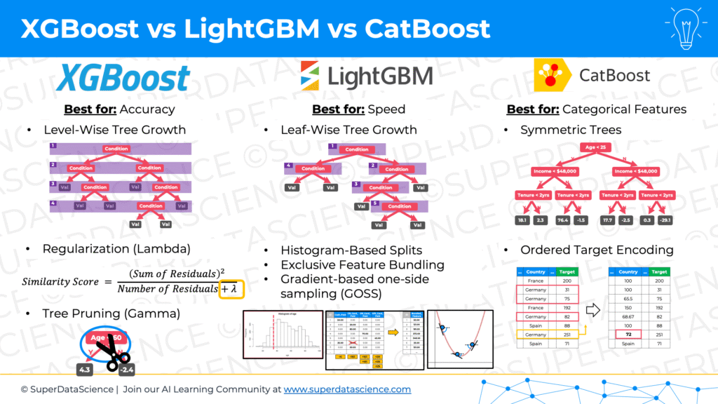
Anyway, so let’s dive back into what is great about eXtreme Gradient Boosting that wasn’t so great in normal Gradient Boosting. So first thing, it uses special kinds of decision trees. The way the decision trees… in normal Gradient Boosting, the way they’re constructed is by greedily, is a technical term, greedily choosing the one split that maximizes the reduction in loss function across all possible splits in each step. It looks for the one, the maximal, the best split. Whereas in XGBoost, it uses something called similarity score, and then it uses a gain calculation. So basically it looks at… Okay, so the way to think about this without going into the mathematics is, how similar are the observations? So we have, let’s say, our first split. We have those 1,000 observations. This is tree number one. We’re looking at the errors. We have those 1,000 errors. How similar are those errors between each other? You calculate similarity score, and then you can have the split in different areas. 

01:14:06

So for each split, and it has an optimized way of not going through all these possible splits. For example, the salary variable. There’s an optimized way that it looks at fewer of them with a certain step, but we’re not going to go into detail on that. But basically it looks at, okay, so if I do the split here, what’s the similarity score on the left of the split and on the right? So if I do a split in this branch, I’ll end up with two leaves. What’s the similarity score of the observation that will end up in the left leaf, and what’s the similarity score between the observations, between among each other, of the ones that will end up on the right leaf? Then you calculate a gain, which is calculated as… you want similarity to be higher. The higher the similarity, the better. 

01:14:53

The gain is calculated as similarity of the left leaf, plus similarity of the right leaf, minus the similarity that you originally had in the leaf that you’re currently splitting. What that does, is if the gain is greater than zero, that means that you’re going to actually gain something from doing the split. If it’s less than zero, you’re not going to gain anything. Also, you want to find the split with the highest gain. So that’s number one. They’re a special kind of decision tree. The way they think about the splits is through similarity scores and gain calculations. 

01:15:25

The second thing is tree pruning. So you build this tree. It builds it depth wise, so it goes from level one to level two where you have your branch. You split into two areas, two splits. Then you split again, you split into four. Then you split again, you split into eight. So it builds it depth wise, and then it prunes it. So pruning is like cutting it, going from the bottom to the top and looking at the gain that you have in each one of the leaves, the gain that we just talked about. And then you have a hyperparameter gamma. So when you’re building XGBoost model, you’ll see a hyperparameter gamma. That is for this pruning. 

01:16:02

So gamma, let’s say you set it to 100, or let’s say you set it to 110, for example, just not to have round numbers. So let’s have 110 as your gain, or your gamma. If your gain in a certain leaf is less than gamma, then you will remove that leaf, and then you’ll go to the next one, go up the branch. If the gain is, again, less than gamma, you’ll remove that leaf, and so on, until you hit a leaf with a gain more than gamma. That way you reduce the size of your decision trees. That’s called tree pruning.

01:16:33

Next one is regularization. XGBoost has built in regularization, so it’s not something you have to add separately. It has built in L1 and L2 regularization, and basically, without going into detail, regularization helps with overfitting. So it helps with preventing overfitting. Next one is sampling. As we discussed earlier, XGBoost or Gradient Boosting, it uses all of the samples. So you have 1,000 samples, there’s no bootstrapping you every time. So the first time, model zero used 1,000 samples, you take the average. With the next model, you take 1, 000 errors and you build that model. The next model, you take 1,000 errors of that model, and so on, and so on, and so on. 

01:17:23

XGBoost has built in sampling of rows. So you can tell it that I don’t want to use 100 rows. There’s a hyperparameter for this. I want to use 80% of the rows. So now each tree will only see a random 80% sample. Let’s say tree number one, we’ll see 80% of the rows, it’ll be built on that. Tree number two, we’ll see a different 80% of the rows be built on that. Tree number three, and so on, so on. Also does sampling of columns. As we discussed with Jon, you can tell it to sample 80% of the columns, or whatever percentage you want, or you can build it on all of them, but there’s a hyperparameter for sampling columns. 

01:17:59

There is a built-in cross-validation, k-fold cross-validation, if you want. Also, without going into detail on the technicalities of this, XGBoost was developed with high scalability and performance in mind. So there are additional optimizations specifically for hardware and for accelerated computing, basically, and also it supports distributed computing to handle very large datasets. So XGBoost was built with all those things in mind, and as a result, it’s very efficient and it allows it to do more optimization cycles in the same period that a different model will do. That’s what makes it so incredibly superior. I think it was actually Francois Chollet, if I’m not mistaken, that said that, “The winning teams are the ones that…” This isn’t Kaggle, but of course the same thing applies in industry. The best models are the ones where you can iterate more times in the same given time, so you want your model to be super efficient, super fast. 

Jon Krohn: 01:19:05

Yeah, it’s super fast. That’s also key for when you get your model into production where it’s ideal, obviously, if your costs are lower, you don’t need as much compute to be able to support lots of users using your model in real time in that production infrastructure. So, valuable for sure. 

Kirill Eremenko: 01:19:22

All right, so that’s XGBoost. Let’s talk about LightGBM, do a quick overview, and CatBoost. Okay, so LightGBM, introduced by a team at Microsoft in 2017, a few years after XGBoost. You can find a paper. The paper is called LightGBM: A Highly Efficient Gradient Boosting Decision Tree. And interesting comment, in 2022, LightGBM was dominant out of the gradient boosted decision trees models among Kagglers. So even already, according to that poll that Francois Chollet did, it was already ahead of XGBoost by 2018. More winning models on Kaggle were using LightGBM. 

01:20:11

So what’s super cool about LightGBM? Well, LightGBM takes what we just discussed, that concept Jon and I just mentioned about more iterations, more cycles, iterative cycles in a given time, takes it to the next level. I don’t have a reference for this, but LightGBM is considered to be, by some blog I read somewhere online, it’s considered to be 20 times faster than XGBoost. So it sacrifices accuracy for speed, and does so consciously and in a few methods, which we’ll talk about now. It sacrifices some accuracy for a huge gain in speed.

01:20:50

Okay, first thing. The biggest, coolest thing about LightGBM that you need to know, is that the trees use histogram-based splits. So think about it, our column, with salaries. We have salaries of 1,000 people, estimated salaries, that we’ve estimated. The salaries can range from zero, somebody who’s currently unemployed, not working, can range to maybe 100… I don’t know what salaries… it could be 200,000. What was the risk salary for somebody doing machine learning at… what’s it called? Netflix? Or Anthropic? 600,000 I saw. Like crazy, to the research- 

Jon Krohn: 01:21:29

Yeah, base pay. 

Kirill Eremenko: 01:21:29

Let’s say for argument’s sake, it goes up to $150,000. But in that range you have 1,000 different values. It can be $67 and $232.23. There’s a huge variability of salary in that. There’s lots of options that salary take. What if you had not 1,000 customers, or you had 10,000 customers? There’s now potentially 10,000 different values, 10,000 places you could split this dataset.

01:21:58

But what if you take all of these salaries and you put them into a histogram, basically you bin them? So you create bins with a $10,000 step. So your first bin is from zero to $10,000. Your second bin is from $10,000 to 20,000, then 20,000 to 30,000, and so on. So you end up, if your salaries are between zero and $150,000, and your bin size is 10,000, you end up with 150 bin. 150? No, you end up with 15 bins, right? 15 bins. 10 bins gets you to 100,000. Yeah, 15 bins total. So you end up with 15 bins, and now all of your observations, all of your customers are put into this histogram or end up in one of the bins. And now what LightGBM does, is it doesn’t split on the salary, it splits on the bins. So now it has only 15 options, or 14. If you have 15 bins, you only have 14 options where to split to make that split for salary. 

01:22:56

It’s so much faster, right? Instead of looking at 1,000 different options, you’re looking at 15. And if you have, let’s say, 10,000 customers, instead of looking at 10,000 options, hypothetically, you can only still look at 15. It doesn’t change. So this histogram-based split, of course, it’s less accurate, of course, you can’t now split somewhere in the middle of a bin. It has to be on the borders of a bin. You can only split at 50,000 or 60 or 70 or 80, you can’t split at $63,000, but you’re sacrificing accuracy. The whole idea behind LightGBM, in my view, is sacrificing accuracy for speed. That’s one of the biggest parts. 

01:23:34

The next one is really fun. A bit more complex, but really fun to understand. It’s called Exclusive Feature Bundling. Basically, this is reducing the number of columns at all costs. At all costs, as in, whatever it takes, let’s reduce the number of columns. The authors of LightGBM, if you read the paper, they say that most of the datasets available in the real world in businesses have sparse data, have sparse columns. A normal column like salary, estimated salary, is a dense column. You’ve estimated salary for every single observation. A sparse column is that column that mostly has zeros. Here and there sometimes it’ll have some value.

01:24:18

I was thinking about this last night of how to illustrate this idea that why would most datasets have sparse columns? Well, let’s look at a couple examples. Let’s say you have a dataset which says, “Okay, these are our 1,000 customers, and you have five sales representatives in your candle store that they can call. And each sales representative has a column, sales rep one, sales rep two, sales rep three. And you’re recording, if a customer called, which sales representative did they speak with, and for how many minutes?” So basically, sales rep one will have number of minutes for each customer they spoke with. It might be five minutes for customer one, it might be 120 minutes for customer number 733, et cetera, et cetera.

01:25:09

But for most customers, it’s going to be zero. There’s no chance a sales representative spoke with… They only spoke with maybe, out of your 1,000 customers, they only spoke with 12 over the course of a month or something like that. And then sales rep two will have values for other customers, and so on. Most of the values in these columns will be zero. 

01:25:32

Let’s look at another example, just to illustrate the point. You could have, for example, trucks. At a mining operation, you have 1,000 trucks and they can only do one of three jobs, or one of five jobs, and the jobs are the columns. So then you would have how much time or how many kilograms of ore did that truck do on that job? And then there could be another column for maintenance. For example, how many minutes did the truck spend on maintenance? And so on. So there can be a lot of columns that have mostly zeros and some values in it. 

Jon Krohn: 01:26:07

Big surprise that our Australian podcast guest is talking about ore mining. 

Kirill Eremenko: 01:26:13

Yes. Yes, that’s true. I actually worked on a project relating to that for six months back at Deloitte. It was really fun to go fly out to the middle of nowhere and be on this analytics project. Really cool. 

Jon Krohn: 01:26:29

Putting an occasional one in a column that’s otherwise all zeros. 

Kirill Eremenko: 01:26:33

Yeah, yeah. But in this case, we’re looking at columns. It’s because it’s easier to talk about regression. Rather than classification columns, we’ll look at columns with continuous variable, continuous values. So that was a second example of a sparse column. You can imagine loss of sparse columns in any kind of industry, like medical datasets, like which doctor this patient saw or procedures they had. You can imagine columns with time sheets of employees and things like that.

01:27:05

Oh, you had a great podcast with the person from Spotify. Remember that podcast? 

Jon Krohn: 01:27:12

Spotify? Oh, yeah. Erik Bernhardsson. The guy- 

Kirill Eremenko: 01:27:17

Erik Bernhardsson. 

Jon Krohn: 01:27:18

… who developed the Spotify [inaudible 01:27:19]- 

Kirill Eremenko: 01:27:19

What episode number was that? That was such a good podcast. I loved when he was talking about… He was talking about sparse columns, because they had a huge spreadsheet or dataset at Spotify where each column is a song and each row is a customer, and each value is how many minutes of that song did that customer listen to it? It’s mostly zeros because you don’t listen to all of the songs. It’s a very sparse dataset. 

Jon Krohn: 01:27:47

Yeah, that was episode number 619. Yeah, it is definitely a great episode with Erik Bernhardsson. He’s an amazing speaker, an amazing technologist, an amazing entrepreneur. 

Kirill Eremenko: 01:27:57

Yeah, I loved that episode. So there’s sparse datasets all over business and industry. We don’t see them that much in practical practice tutorials or examples, and that’s why it’s important to do labs, like live labs or workshops, which expose you to these kind of real world scenarios. But they exist and they’re all over the place.

01:28:17

What LightGBM does, is it… we’re not going to go into detail on this, but basically it combines sparse columns into fewer columns. You might have 100 sparse columns. It has a method for combining them, even if they’re talking about different things. One could be talking about salaries, another could be talking about kilograms, another one could be talking about, I don’t know, time. It has a way to combine them into, from 100, you might cut it down to five or four columns. And that’s very beneficial for Gradient Boosting decision trees and other methods. It really speeds up the decision tree building process. 

01:28:57

We talked about sacrificing accuracy. The way it sacrifices accuracy is that in some cases it will combine… like in some cases, a row might be more populated than other rows. It might have values in a lot of these columns. Well, LightGBM will cut out, drop some of the values in order to achieve this combination. So we’ll reduce accuracy by allowing data loss, but at the same time, the speed will go up. So that’s called Exclusive Feature Bundling.

Jon Krohn: 01:29:27

Nice. 

Kirill Eremenko: 01:29:28

Good. Cool. Next one is Gradient-Based One-Side Sampling. This is a really cool one. 

Jon Krohn: 01:29:33

Oh, yeah. When you say next one, it’s another… We’ve had a few of the key ideas behind LightGBM, which also, the etymology of that Light Gradient-Boosting Machine is what GBM stands for there. 

Kirill Eremenko: 01:29:48

Oh, great. Yeah, yeah, that’s right. 

Jon Krohn: 01:29:51

So Light, the idea that it’s so much faster, 20 times faster, as you’ve said, relative to XGBoost, which already was super fast relative to the vanilla Gradient Boosting that you went into. So you have been enumerating most recently the main ideas behind how LightGBM is 20 times faster than XGBoost. The first one was histogram-based splits. The second one was Exclusive Feature Bundling. And now you’re going to go into a third one, which is… 

Kirill Eremenko: 01:30:23

Gradient-Based One-Side Sampling, or GOSS, G-O-S-S, for short. It sounds complex. It’s actually very simple. Based on what we discussed, it’ll be very easy to get your head around it. Basically, once you’re building a decision tree, you have the gradients that you want to predict and you want to reduce your loss function. Instead of building a decision tree for all of the observations, right? Or instead of sampling 80% at random like XGBoost can do, why don’t we be smart about it and why don’t we look at these gradients? So we have 1000 gradients. Let’s order them from largest to smallest, and let’s take the top 20%, so top 200 gradients and use them plus of the remaining. So that’s a hyperparameter A and then there’s a hyperparameter, we’ll call it B. Then you have the remaining 80%, the remaining 800 gradients of them. Just to have a representative dataset, take a random 10%. So take a random 80. So as a result, you will have 200 observations with the highest gradient plus 80 observations random ones with lower gradients, and you have now a sample of 280. And you’re going to build a decision tree based on that. 

01:31:46

And why is that? Of course, you’re sacrificing accuracy. You’re using fewer rows. But you’re gaining a lot of speed, and you’re not sacrificing that much accuracy because you’re taking the top 20% gradients that you need to improve anyway. So why worry about the 80-20 rule, right? Let’s improve these 20% gradients ’cause they’re the highest. So that’s what gradient-based, and it’s called one side sampling because you’re taking the highest 20% of the gradients. So in total, if your parameters are 20% and 10%, you’ll end up with 28% of your dataset. So that’s gradient based, one side sampling, that’s the third main idea behind LightGBM. And the fourth one is called leaf-wise tree growth. So XGBoost and normal grain boosting have depth-wise tree growth. So you start at level one, the branches, you have an if-else condition. Then you have two branches, then you split each one of those into four. 

01:32:40

So you get four branches in the total. Then you split that, you get eight and so on. So it keeps going from top to bottom. At each level, this splits on both sides, on all of the sides. Whereas LightGBM approaches this in a smarter way, it’s like, “Why should we build such a massive decision tree? Let’s do one leaf at a time.” So at the start, you split into two branches. Then you have one on each side, right? So now, instead of splitting both, you only split the one that will give you the best result, the best improvement for your model. So the left side or the right side. Let’s say you split the right side, now, you have three leaves in total instead of four. Now, you split one of those leaves. 

01:33:25

Now, after this split, let’s say you split the most bottom on the left, right now, you’ll have four leaves in total. So you’re adding one leaf at a time, increasing the number of leaves by one because you’re splitting one leaf at a time. Whereas in the other one, in the XGBoost, you’re doubling your number of leaves every time. And the way that this can be beneficial is in LightGBM, you’ll have a parameter of maximum number of leaves. So your maximum number of leaves might be like 30. And so instead of getting there by doubling every time, you’re getting there in a more conscious way. And your decision tree will look very different because you’re using the best splits every time. So that was the fourth and final main idea behind LightGBM that makes it sacrifice a bit of accuracy for a huge gain in speed. 

Jon Krohn: 01:34:14

Nicely done, Kirill. You clearly know this stuff well. All right, so we’ve had of the specialized real-world Gradient Boosting approaches that we see lots of winning competitions that people talk about. Absolutely, XGBoost, LightGBM more recently in the last couple of years. And the final one, CatBoost is one to definitely talk about. And that is also actually one. I’ve done a standalone episode on CatBoost before.

Kirill Eremenko: 01:34:39

Oh, wow. Cool. 

Jon Krohn: 01:34:41

Yeah. Episode number 694. It was just a Five-Minute Friday episode. You understand it a lot better than I do, though. I need notes. 

Kirill Eremenko: 01:34:49

Let’s see. Let’s see. Please correct me if you find anything out of order. All right. So let’s talk about CatBoost. CatBoost Stands for Categorical Boosting. It was introduced by a team at Yandex in 2017. A paper is called CatBoost, unbiased boosting with categorical features. If you want to have nightmares of mathematical formulas, have a look at that paper. It is so heavy on math. So let’s go through the main ideas right now. And there’s only just two main ideas that I wanted to highlight. There’s, of course, more to the algorithm, but these are two main ideas. The name categorical boosting is that it deals very well with categorical features. So if you have features, columns in your dataset that are categorical, it handles them automatically. A quick note is that LightGBM also handles… So XGBoost doesn’t handle them automatically, you need to one-hot encoding.

01:35:49

LightGBM handles categorical variables automatically. Probably avoid doing one-hot encoding with LightGBM. What you need to do with LightGBM is you need to convert your categorical variables to integers and point a LightGBM at the categorical variables and it will deal with them, but it’s not as good as CatBoost. So CatBoost is extremely adept at dealing with categorical variables and it does it automatically on the fly. How does it do it? Well, let’s talk about one-hot encoding. Let’s say we have a dataset with your customers, and your 1000 customers are from two different countries. They’re from the UK and from France, right? So you have a column where it says country and it’s UK, France. UK, France, France, France, UK and so on. So what you’re going to do with one-hot encoding is you’re going to replace that column because machines, normally, can’t deal with categorical variables like words. So you want to put numbers in there. 

01:36:54

So you’re going to create one-hot encoded columns, basically dummy variables. You’re going to replace, you create two columns, one for UK and one for France. And so whenever the customer is from UK, it’ll be one in the UK column, zero in the France column. And whenever the customer is from France, it’ll be zero in the UK column, one in the France column. And then actually, you will drop the second column. You want to avoid something called the dummy variable trap because one column is enough to encode two categories. So you’ll just have one column, for UK one or zero, which means in France. But if you have, let’s say three countries, France, UK, Germany, you will have two one-hot encoded columns. If you have 10 countries, you will have nine one-hot encoded columns or dummy variables.

01:37:41

And as you can see, as the number of categories grows, the number of columns explodes. And that is very bad for decision trees because they have to think about more columns which they need to consider. That’s kind of the opposite of what LightGBM was doing by combining sparse columns. So that can be bad for decision trees. Also, there’s other reasons why one-hot encoding is not great for decision trees. For example, it’s hard to assess the importance of the feature country. Like you’ll end up with, let’s say, nine columns for different countries. You can assess how important is Germany or how important is France, yes or no in your final result. But it’s hard to assess how important is country overall. Another reason that it’s bad is, for example, for decision trees, if you split your countries or your categories into different columns with one-hot encoding, you can’t make a split in your tree.

01:38:39

Let’s say the if-else condition, you can only say, “Is it France, yes or no? Is it UK, yes or no? Is it Germany, yes or no?” You can’t say. ” If it is UK or Germany, go left. If it is France or Monaco go, right?” You can’t do that. So it limits the splits, the decision trees can do. Also, you get loss of ordinality. Let’s say you have a categorical column with high school bachelor, master’s, or PhD degrees. If you split into one-hot encoded columns, there’s no longer that ordinality that high school comes before bachelor, bachelor comes before masters, masters come before PhD. You’ve lost that data, that information and so some other things. So basically, there’s reasons why one-hot encoding is not the best for decision trees. Just as a note, one-hot encoding is actually a great method for certain algorithms such as linear regression algorithms and algorithms based on dot product, I think.

01:39:33

That’s where it works really well, like neural networks. That’s where one-hot encoding is very, very relevant, works well, et cetera. Decision trees, not so much. So there’s a different approach to how you can… There’s actually many ways how you can encode categorical variables, it’s just one-hot encoding is the one we most of the time use and that’s why we’re so familiar with it. There’s an approach called target encoding, and it wasn’t introduced… It’s separate to CatBoost. CatBoost uses a special type of target encoding. But in general, what target encoding does is you take your column, let’s say, we have Germany, France, and the UK in our country column for our customers. And then you look at the target variable, and the target variable is how much did they spend in your store. So the “What we’ve been predicting this whole time?” 

01:40:20

For target encoding, the simplest way of doing it is you take all of the rows that have Germany and you take the average of your target, let’s say it’s $57.32. Then you take all of the rows that have France and you take the average of your target, let’s say it’s $98. And take your older rows that have UK and you take the average of your target, which could be $125. And then in your categorical column, you could replace the word Germany with $57.33, whatever it was. Let me write that down, 57 and 33 for Germany. For France, you replace it with whatever we said, I forgot. So let’s say $92.50. And for UK, you replace it with $125. It’s a bit mind-blowing when you think about it because you’re replacing words or categories with continuous variables. The average of your target is mind-blowing for that reason. Well, yeah, the second reason mind-blowing is your… Well, we’ll get to that in a second. 

01:41:29

So why are we replacing categories with continuous variables? Like instead of Germany, it’s $57.33. France is 92.50, UK is 125. Well, it’s called target encoding because now, you’re taking and substituting the category for the relationship that the category has to the target. So there’s clear relationship that Germany has a lower average target than France, and that has a lower average target than the UK. And all you’re doing is you’re taking the average of your target and it’s substituting the words of the category with that average. And the one thing to remember about machine learning is it doesn’t have to be perfect as long as it works. And this works, this really works and helps you split your decision trees better. 

01:42:18

One thing that you might be wondering and rightly so is that “Hey, but we’re taking the target and we’re putting the value from what we’re about to predict into our features.” So we have, it’s called data leakage, right? So you’re leaking information that you want to predict from your dependent variable into your independent variables using target encoding. And there’s certain ways of combating that. For example, there’s k-fold target encoding, there’s weighted target encoding, there’s k-fold weighted target encoding. We’re not going to go into detail on that, we talk about that in depth in the course. But there are ways of combating that and reducing the data leakage to some extent. And this is where we get to CatBoost. The way that CatBoost deals with this problem of data leakage is it looks at one of two things.

01:43:13

If your data has a timestamp column, basically a column that says in which order these observations were recorded, then it will use that, it will order your data based on the timestamp column or based on the time data, whatever you have, from the earliest to the latest. And so basically, what it will always do is it will take a row. For example, let’s say row number 50 is France, so it will take the average of all of the rows that had France before it. So from row 1 to row 49, it’ll look at all of the rows that have France and it’ll take the average of the target for those 49 rows and put it as the target encoding for France in row 50. And then it’ll go to row 51, and let’s say it says Germany. So for that Germany, for row 51, it will look at all of the rows between row 1, row 50 that had Germany as the category. It’ll look at the average of the target and it’ll use that average as a target encoding in row 51. 

01:44:16

So you’re never looking at the value of the actual target of the row you’re encoding, you’re always looking at the rows that came earlier. And you’re not leaking data because those rows actually came earlier in real life. There’s a cause and effect. They happened earlier, so you’re fine. You’re allowed to look at that data in your target encoding. So that’s the simplest option. Second option is if your data does not have a timestamp column or does not have some order in which the columns came. What CatBoost will do is it will shuffle your rows randomly and it’ll do the same thing. You’ll basically pretend that there is a timestamp column. And it’ll go down, and it will look at the previous rows and use the average as a target encoding for this row, and the average will be calculated on all the previous rows. It’s a bit more complex than that, we won’t go into detail on that. 

01:45:10

There’s four permutations, so it shuffles your data four times. And then it uses these permutations, three of them in one way, the other one in a separate way. So we won’t go into detail on that. But the point is it uses something called ordered target encoding, and it replaces a categorical variable with that. There still potentially can be data leakage to some extent with any kind of target encoding, especially if you’re shuffling rather than using a data timestamp column. But again, the big takeaway for me, anyway, from all of these Gradient Boosting methods and their optimization techniques is that it doesn’t matter if it’s not perfect, machine learning doesn’t have to be perfect. It has to give it results. 

01:45:55

And even if there’s some data leakage, who cares? If your model works. It’s not perfect, but it works. It gets you the result. It works on the test dataset, it passes your k-fold cross validation. Who cares that there’s a bit of data leakage, or a bit of loss of data, or a bit of inaccuracy? As long as it works. And that’s what these Gradient Boosting methods is so good at is it that trade off of, “All right. We have Gradient Boosting, which is theoretical, what’s the point of that?” Let’s do some trade-offs. Let’s make it faster. Less perfect, but faster. And boom, we get amazing results. 

Jon Krohn: 01:46:27

Wow. Yeah, you definitely know this way better than I do. I just learned a ton about CatBoost. So all of those are the main ideas for why CatBoost works so well for categorical data. As a Gradient Boosting algorithm, I think it’s the obvious go-to choice for working with categorical features. And yeah, so you talked about how it doesn’t use the typical one-hot encoding that you would get with a regression model, you combat data leakage, you have all those permutations. And yeah, that’s how it’s so powerful. 

Kirill Eremenko: 01:47:05

Perfect. Yeah, exactly. And the second reason why CatBoost is powerful is that it can… Excuse me. The main idea about CatBoost is it’s very straightforward, very simple. Yeah. 

Jon Krohn: 01:47:17

Like other than the categorical part. So like [inaudible 01:47:19]- 

Kirill Eremenko: 01:47:19

Yeah, other than the categorical. So- 

Jon Krohn: 01:47:20

Yeah, yeah.

Kirill Eremenko: 01:47:21

So that was the main thing. That’s why it’s called CatBoost. That’s how it works with categorical variables, it’s the big one. But in addition, one that they threw in there is symmetric trees. You can use symmetric trees. You can build your own algorithm, brain boosting to symmetric trees. They decided to use symmetric trees because they’re faster. So just imagine a normal tree as we discussed, you have a split at the top. Then it goes down one way, so you can split at salary at $47,000, for example. Then you go left, you split by age at 25 or 45 years old, whatever it is like the decision tree decide. But if you go right from the salary, you’ll be splitting by, “Do they have a loyalty membership?” And then you go further down. So the tree spreads and the branches are independent, they do whatever they want kind of thing.

01:48:05

That’s a traditional tree. With a symmetric tree, every time you split, the branches will make further splits on the same variable, on the same condition. So imagine, at the top, you have is this person earning less than $45,000. Okay. So if it’s a yes, then you go left. And the next condition you’ll find on the left is, for example, “Is this person younger than 25 years old?” Well, if you were going to go right from the original one about the salary, if you’re going to go right, well, the split on the right is going to be exactly the same. It’s going to be, “Is their age less than 25?” Now, from the age is less 25, you’ll get two splits on each side. So you’ll have four leaves after that, right? And there, the splits, let’s say, “Do they have a loyalty program, yes or no?”

01:49:01

Each one of them will be a yes or no loyalty program. And then from there you’ll have eight splits, the next time, so it’ll double again. But let’s say you’re using a different variable now, let’s say you have a variable on the, I don’t know. Let’s say, we’ve done age, salary, the distance to your… Or how much time they spend on your online store? So now, it’s going to be, “Have they spent less than 15 minutes on the online store in the past month?” Well, all eight will have exactly the same condition. So you’re building the decision tree in a way that every next level horizontally across the tree is the same exact condition. And why is that good? Well, of course, the tree becomes weaker because of that. 

01:49:51

It’s a weaker learner than a traditional decision tree because it has less flexibility. But guess what? In ensemble methods, we prefer weak learner. So it’s actually not a bad thing that it becomes weaker. And the second thing, which is the main benefit is that it becomes much faster during inference. Not during training, you still have to build the tree during training, but during inference it becomes much faster. And the way to think about it is now, let’s say, you have four levels. So at the beginning you have a question about salary. The second question is about age. The third question is about loyalty program. And on the fourth level is about how much time they spend less than 15 minutes on your website or not, so time on the website.

01:50:34

So now, because all of the levels are the same, you can take, let’s say a new customer comes to your store, you can take those exact variables, salary, age, loyalty program, “Yes or no?” and time on the website. You put them into one vector and so it’s a vector where they’ve got their salary, however much they’re making. Their age, whatever it is. If they’re loyalty, yes or no, one or zero. And how much time they spend on the website. And now, instead of going down through this decision tree and every time deciding what yes or no, yes or no, yes or no… So like making all these comparisons, you have to make one comparison. You take the vector that you’ve built for this customer, and you compare it to the vector of conditions. 

01:51:19

So the vector of conditions will be the salary that you’re splitting on, let’s say $47,000. The age, let’s say 25 years old. Do they have a loyalty program? There’ll be a one for a yes and the amount of minutes, let’s say 15 minutes. So you’ll have a vector of conditions. You just have to compare the original vector to the vector of conditions, and you’ll get a vector of ones and zeros. Where did the condition, was it correct, was it not correct? Because all of the splits on the each level are the same. Whichever way you go, there is no difference in the splits. So you just need to do this correct… Check once. And is your vector for this customer… Then you do the mathematical operation less than the vector that you are looking at, the vector of conditions and then you’ll get a result. It’s like one, zero, one, zero, for example. And then from there, you’ll know that the answer for that customer is $76.40. 

01:52:13

So it speeds up inference, meaning that instead of doing… Before with a traditional tree, you will have to do up to X comparisons, where X is the maximum depth of your tree. With this one, with CatBoost, with symmetric trees, you just have to do one comparison. You just compare one vector to another and that’s it. And then you get your result very quickly. So if you have an application where your speed at inference is important, whether it’s like real-time analytics or I don’t know, some gaming application, or something that has to happen fast in inference, then you might consider using symmetric trees or specifically CatBoost. 

Jon Krohn: 01:52:57

Nice. So that was obviously a ton of information. You have Kirill really pushed the boat out on providing tons of technical content in podcast format. It’s been extremely well received so far. I thought it was going to be risky when you started doing that earlier this year for transformer architectures, but people have loved these episodes. So thank you for all of that detail. I understand that you’re going to include a cheat sheet in the show notes- 

Kirill Eremenko: 01:53:25

That’s right. 

Jon Krohn: 01:53:25

… for these three main Gradient Boosting approaches. XGBoost, LightGBM, and CatBoost. You’ll have a cheat sheet from your SuperDataScience exclusive course made available. 

Kirill Eremenko: 01:53:38

That’s right. That’s right. It’ll be a cheat sheet, a one-pager that compares all three models side by side. XGBoost, LightGBM, CatBoost. It’s from one of the tutorials. Happy to share it. It’ll be in the show notes. Feel free to download it and keep it as a memento of this episode hanging out on the wall or something like that. And it has all the summary of everything that we discussed. 

Jon Krohn: 01:53:56

Nice. So other than www.superdatascience.com/level2, where that’s just the integer two at the end as opposed to straight characters. Level two, the number two. 

Kirill Eremenko: 01:54:11

Yep. 

Jon Krohn: 01:54:12

Superdatascience.com/level2, other than that, how should listeners reach out to you or learn more after this episode? 

Kirill Eremenko: 01:54:21

Sure, I’ll mention that just now. I just wanted to say with this course… So in the course we talk about everything. We talked about today in detail, of course, visuals and stuff like that. In addition to those three methods, we talk a lot about… Of course, you’ll learn additional things like one-hot encoding, k-fold cross-validation, bias-variance tradeoff, hyperparameter optimization techniques like grid search, target encoding, AdaBoost. And there’s going to be lots of practice. Hadelin walks through each one of these models, XGBoosts, LightGBM, and CatBoost for both regression and classification. For regression, he uses an insurance dataset. And you get to see how these models perform differently on the same dataset. And for classification, he uses a churn dataset for customers, whether they will churn or not from a company. And again, you’ll see how these three models perform differently on that dataset. 

01:55:10

And of course, once you get your membership at SuperDataScience, you get access to this course exclusive on SuperDataScience to the Large Language Models A-Z course, which we released recently. Also, exclusive to SupeDataScience, not available anywhere else. Plus, at the moment we’re doing two live labs per month plus a career session. We’re gearing up to ramp it up to, my goal is four live labs per month starting next few months. And basically, that’s a live experience where you get a coach, an experienced machine learning, AI, visualization practitioner who walks you through creating, solving some real-world business challenges. And I think what we’ve heard from our students, it’s the main thing that helps them get jobs. One of the biggest bonuses that helps them get jobs is live trainings like that. 

01:56:00

So that was a bit of a promotion for SuperDataScience. And in order to find me, you can connect on LinkedIn. But to be completely open about it, I don’t go on social media these days often, the best way to connect with me would be in SuperDataScience. We have a community, people ask questions, chat with each other, and I’m there every week, several times per week. And my goal is to be able to answer everybody and connect with everybody there.

Jon Krohn: 01:56:29

Nice. Thanks, Kirill. Well, it’s great to know that they have access to you through the www.superdatascience.com platform. It sounds like a very vibrant place indeed and increasingly exclusive content like this Gradient Boosting course available just there. Super Kirill, thank you so much for joining us yet again for another super technical episode. I’m sure the audience loved it, and I wouldn’t be surprised if you weren’t back again doing another one of these sometime soon. 

Kirill Eremenko: 01:57:00

Fantastic, Jon. Thanks again for having me. It was a lot of fun. 

Jon Krohn: 01:57:09

Another incredibly rich technical episode from Kirill. He sure knows how to explain technical content well and even have a bit of fun while doing it. In today’s episode, Kirill fill us in on decision trees, bagging, random forests, AdaBoost, and the three leading Gradient Boosting algorithms. XGBoost, LightGBM, and CatBoost. As always, you can get all the show notes including the transcript for this episode, the video recording, any materials mentioned on the show, the URLs for Kirill’s social media profiles, as well as my own at www.superdatascience.com/771. And if you’d like to meet in person as opposed to just through social media, next week I will be at the Data Universe conference at the massive Javits Center in New York City. That’s April 10th and 11th next week. I’ll be giving a talk on generative AI, and we’ll also be walking around interviewing attendees to capture what you think of this massive conference.

01:58:02

All right. Thanks to my colleagues at Nebula for supporting me while I create content like this SuperDataScience episode for you. And thanks of course to Ivana, Mario, Natalie, Serg, Sylvia, Zara, and Kirill on the Super Data Science team for producing another extremely illuminating episode for us today. For enabling that super team to create this free podcast for you, we are deeply grateful to our sponsors. You can support this show by checking out our sponsors’ links, which are in the show notes. And if you yourself are interested in sponsoring an upcoming episode, you can get the details on how by making your way to jonkrohn.com/podcast. 

01:58:32

Otherwise, please share, review, subscribe, and all that good stuff. But most importantly, just keep on tuning in. I’m so grateful to have you listening and hope I can continue to make episodes you love for years and years to come. Until next time. Keep on rocking it out there, and I’m looking forward to enjoying another round of the Super Data Science Podcast with you very soon.