Organising data. Manipulating data. Tidying, cleaning, mining. Munging data? There are many ways to describe the steps to create “clean” or “tidy” data for analysis, visualisation or to apply machine learning techniques. My preferred term is the “wrangling” of data as it conjures the image of a cowboy twirling a lasso on horseback (not this sun-deficient geek with poor posture hunched over a laptop).
I perform a common number of steps when wrangling data. Here I outline such steps using R, then show an equivalent code in Python. The code is PC-specific (those on Macs will need to make minor adjustments). The following data wrangling steps will be covered:
- Load packages/libraries
- Load raw data
- Bind rows
- Select and rename columns
- Change data types
- Create datetimes
- Remove duplicate rows
- Group by, filter and summarise
- Join data frames
- Visualise data
- Save tidy data
To follow along, here is the link to the R code and to the Python code.
We start with raw data and will end with tidy data. We need some data.
The raw data
Kaggle is an excellent repository of open-source data. I am using the Crimes in Chicago dataset. The data reports the incidents of crime (not including murders) that occurred in the City of Chicago from 2001 to present. Each crime event has a datetime stamp and the Beat, District and Ward geographic area of occurrence. One field indicates when an arrest occurred, and another whether the crime was a domestic incident.
Let’s dive into the dataset starting with R.
Part 1 – R
Load libraries
#### Libraries### Load librarieslibrary(readr)suppressPackageStartupMessages(library(dplyr))suppressPackageStartupMessages(library(lubridate))library(ggplot2)There are four packages I will use.
readr provides functions to easily load CSV data. dplyr is the workhorse of data wrangling. lubridate provides functions to extract values from datetimes. ggplot2 is the much-loved data visualisation library. When you have a moment, Google “tidyverse”.Load raw data
I previously downloaded the four CSV files from Kaggle by selecting the file then clicking on “Download File”.


Each file is in my PC’s local directory where I store open datasets (with path
C:UsersMuhsin KarimDocumentsDatasource_datakagglecrimes_in_chicago). The code shows how I change the working directory so that R knows where to look for the data. Use forward slashes when setting the directory.#### Get raw data## Set working directory#! Change to your working directory here !#setwd("C:/Users/Muhsin Karim/Documents/Data/raw_data/kaggle/crimes_in_chicago")## Load in each filedf1 <- read_csv("Chicago_Crimes_2001_to_2004.csv")df2 <- read_csv("Chicago_Crimes_2005_to_2007.csv")df3 <- read_csv("Chicago_Crimes_2008_to_2011.csv")df4 <- read_csv("Chicago_Crimes_2012_to_2017.csv")Load data with the
read_csv() function (readr package). There are multiple ways to read in CSVs – I use read_csv() because it is faster to load, does not convert columns of data to factors and is a simple one line code. Choose simple.Bind rows
I loaded each CSV file as a data frame. They are bound together (stacked by rows) to create one large data frame of 7,941,285 rows [1]. The separate data frames are removed from memory.
## Bind rowsdf <- rbind(df1, df2, df3, df4)rm(df1, df2, df3, df4)Select and rename columns
You may not want to include all the columns loaded. The first column is a mystery to me – R assigned it the column name “X1”. I do not need it. I will also remove the “IUCR”, “X Coordinate” and “Y Coordinate” columns using the
select() function from the dplyr package.#### Format data## Remove columnsdf <- df %>% select(-X1, -IUCR, -'X Coordinate', -'Y Coordinate', -Location)## Rename columncolnames(df)[colnames(df) == "Date"] <- "Datetime"Using base R, the “Date” column when the crime occurred is renamed to “Datetime”, because it is actually a datetime and I am pedantic when it comes to such things.
Change data types
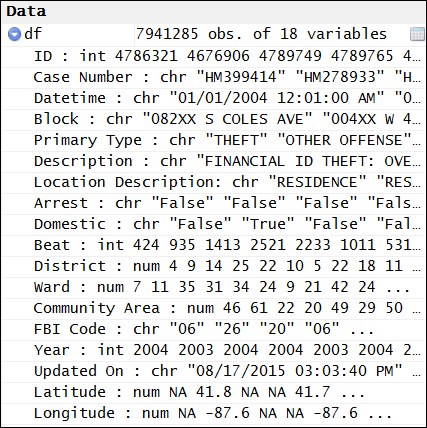
type int (integer). I want “ID” as a character. Functions
as.character(), as.numeric(), as.POSIXct(), etc allow easy coercion of a data column to a different data type.### Change data typesdf$ID <- as.character(df$ID)Create datetimes
Coercing data from a character to datetime is a pain. I have performed this step multiple times yet it remains just as tedious as my first time [2]. I may just be recalling bitter memories each time I have to do it.
An example of a string from the “Datetime” column is “01/01/2004 12:01:00 AM”. Which value is the month? Let’s use another example, “06/20/2004 11:00:00 AM”. Thus, the first value denotes the month (“06”, June) and the second is the day (the 20th).
In order to convert the string to datetime using the as.POSIXct() function, R needs to know the format of the string. Here is a table of datetime format codes and their meaning.
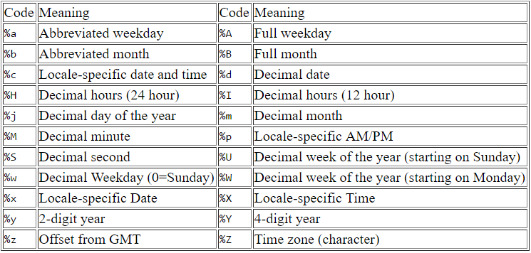
The “%m” denotes the decimal month (e.g. “06”), “%d” is the decimal date (e.g. “20”), %Y is the 4-digit year (e.g. “2004”), etc. As a rough attempt, the format for our example string (“06/20/2004 11:00:00 AM”) would be something like “%m/%d/%Y %H:%M:%S”.
There are two considerations with our strings. First, the strings have “AM” or “PM”. Use “%p” for locale-specific AM/PM. However the format “%m/%d/%Y %H:%M:%S %p” will not produce the correctly converted datetime. Rather, it will produce the hour in 12 hour time, not 24 hour time making AM and PM hours indistinguishable.
The second consideration is to use of “%I” rather than “%H”. “%I” specifies decimal hours from 01-12, matching the current format of our strings. Thus, the correct format for use in as.POSIXct() is “%m/%d/%Y %I:%M:%S %p”. Now that the “Dateime” data is of type dateime, functions from the lubridate library derive the month name, year and hour of when the crime occurred.
### Create datetimesdf$Datetime <- as.POSIXct(df$Datetime, format="%m/%d/%Y %I:%M:%S %p")df$'Updated On' <- as.POSIXct(df$'Updated On', format="%m/%d/%Y %I:%M:%S %p")#### Create columns### Create columns from datetime## Month namedf$Month <- NAdf$Month <- months(df$Datetime)## Monthdf$'Month Value' <- NAdf$'Month Value' <- month(df$Datetime)## Year Monthdf$'Year Value' <- NAdf$'Year Value' <- paste(df$Year, sprintf("%02d", df$'Month Value'), sep="-"))## Hourdf$Hour <- NAdf$Hour <- hour(df$Datetime)Remove duplicate rows
Ideally, the dataset should contain one row per unique crime committed. Duplicates may exist in a dataset for different reasons such as data entry error or updates to existing logged crimes [3]. Each crime has an “ID” and “Case Number”. I concatenated “ID” and “Case Number” to create a unique identifier for when there are multiple IDs per Case Number and vice versa. The data frame is ordered by the “Updated On” datetime in descending order, placing the most recently updated rows at the top.
#### Remove duplicates## Create unique identifierdf$Identifier <- NAdf$Identifier <- paste(df$ID, df$'Case Number', sep="-")## Remove duplicatesdf <- df[order(df$'Updated On', decreasing= T), ]df <- df[-which(duplicated(df$Identifier)), ]I want to remove any duplicate identifiers to have a unique crime per row. When duplicate identifiers are found, the function ignores the first occurrence then removes the rows of subsequent duplicate identifiers from the data frame. The most recently updated records of the duplicate identifiers remain since these are at the top of the data frame (previously sorted by “Updated On”).
Group by, filter and summarise
I want to set up a goal to motivate the next few data wrangling steps. To calculate the frequency of a crime per month, I sum the rows for that crime in the data frame (I am assuming that each row is a uniquely recorded crime using unique identifiers). The crime frequency alone does not factor in the number of total crimes for a given grouping (e.g. per month or per District). Let’s create a column that indicates the crime rate for each crime type.
In this example, crime rate is the frequency of a given crime per group (e.g. a month, a District) out of all crimes in the same group. A District may have experienced an increase in the frequency of theft over time. However, the theft crime rate could be a flat line and not increasing at all with respect to all crimes.
The crime rate per month and District will be calculated. I need two sets of values for the crime rate:
- For each crime type, the number of crimes per month and District (numerators)
- The number of crimes per month and District (denominators).
I will calculate crime rate per month and District using group by, filter and summarise functions.
I make heavy use of the trusty workhorse dplyr package. First, the numerator values. I filter out any rows from data frame “df” with NA (no available data) “Datetime”, “District” and “Primary Type” (crime type). I group the data by the three columns “Year Month”, “District” and “Primary Type”, then dplyr summarises the row counts for each distinct combination of these three columns. Counting the rows for each “Year Month”, “District” and “Primary Type” combination is equivalent to counting the frequency of crimes per group.
#### Crime rate per month per District## Get crime counts for each Primary TypedfDistrict <- df %>% filter(!is.na(Datetime)) %>% filter(!is.na(District)) %>% filter(!is.na('Primary Type)) %>% group_by('Year Month', District, 'Primary Type') %>% summarise(Numerator=n())dfDistrict$ID <- NAdfDistrict$ID <- paste(dfDistrict$'Year Month', dfDistrict$District, sep=" ")An “ID” column is created using the “Year Month” and “District” column in the numerator data frame “dfDistrict”. This column is required to join to the data frame containing the denominator values.
I calculate the denominators in a similar way, except the data is not grouped using “Primary Type”. “Primary Type” is not used in order to get the crime counts per month and District only. The “ID” is created using “Year Month” and “District” as before.
## Get crime counts for each monthdfMonthly <- df %>% filter(!is.na(Datetime)) %>% # to match Python filter(!is.na(District)) %>% group_by('Year Month', District) %>% summarise(Denominator=n())dfMonthly$ID <- NAdfMonthly$ID <- paste(dfMonthly$'Year Month', dfMonthly$District, sep=" ")dfMonthly <- dfMonthly[ , c("ID", "Denominator")]We have a numerator data frame
dfDistrict and a denominator data frame dfMonthly, both with ID columns. I will use the ID columns to join the two data frames together.Join data frames
dplyr joins the numerator and denominator data frames using the ID column.
## Join to get numerator and denominator togetherdfJoin <- left_join(dfDistrict, dfMonthly, by="ID")dfJoin$'Crime Rate' <- NAdfJoin$'Crime Rate' <- dfJoin$Numerator/dfJoin$Denominator * 100The image below shows “Numerator” and “Denominator” columns with the “ID” column in-between. There is a unique numerator for each group of “Year Month”, “District” and “Primary Type” (left-side) and duplicated denominators across rows for “Year Month” and “District” groups (right-side).
I calculate the crime rate by dividing the values of the Numerator column by the values of the Denominator column, then multiplying by 100 to express crime rate as a percentage.

Visualise data
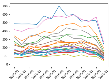
Let’s take a quick look at our grouped data. Here I have a plot of the theft crime frequency from January 2016 onwards. The two lines closest to the top are District 1 (red) and District 18 (blue). The frequency of theft peaks in District 1 in July 2016.
#### Visualization## Prepare data frame for Theft form 2016dfPrimaryType <- dfJoin[dfJoin$'Primary Type'=="THEFT", ]dfPrimaryType <- dfPrimaryType[dfPrimaryType$'Year Month'>"2015-12", ]dfPrimaryType$District <- as.factor(dfPrimaryType$District)### Plots## Crime frequency - theftp <- ggplot(dfPrimaryType, aes('Year Month', Numerator, group=District, color=District)) + geom_line() + theme(axis.text.x=element_text(angle=45, hjust=1, vjust=0.5))print(p)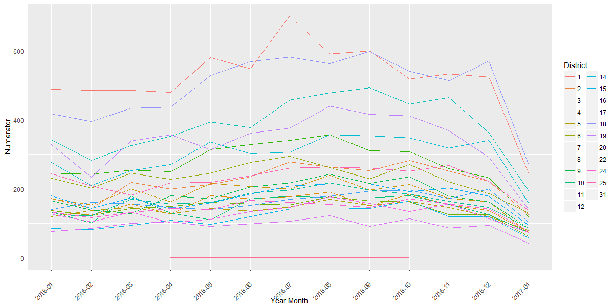
The corresponding plot for theft crime rate is below. At the very top are two points from District 31 with 100% crime rate. However, there are only two logged crime incidents, in May and October 2016, so ignore this line. Consider District 1 (red line) – there were more thefts based on frequency during July 2016 (above plot). Yet the crime rate is flat across the months (below plot), suggesting that the frequency of theft per month (numerator) is in proportion to the total number of crimes per month (denominator), resulting in a flat crime rate across months. I intend to look for any crime rate peaks over a greater stretch of time for different crimes, but I will not cover that here.
## Crime rate - theftq <- ggplot(dfPrimaryType, aes('Year Month', 'Crime Rate', group=District, color=District)) + geom_line() + theme(axis.text.x=element_text(angle=45, hjust=1, vjust=0.5))print(q)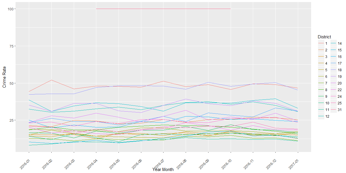
Save tidy data
#### Save tidy datasetwd("C:/Users?Mushin Karim/Documents/Data/tidy_data/crimes_in_chicago")write.csv(df, file="tidy_R.csv", row.names=F)save(df, file="tidy.Rdata")save(dfJoin, file="join.Rdata")The final step is to save the tidy data.
write.csv() will save the data as a CSV file. I have also saved the data as an R object. In addition, I save the “dfJoin” data frame as an R object.The R data wrangling script is complete! Now, Python.
Part 2 – Python
Here I provide Python code equivalent to the R code. The goal is to produce the same tidy data CSV file as produced by R. With this goal in mind, I will compare Python to R.
Load packages
#### Packages## Load packagesimport osimport pandas as pdimport matplotlib.pyplot as pltI use three Python packages. “os” allows the changing of directories. “pandas” provides data wrangling functionality including group by, merging and join methods akin to R’s dplyr package. “matplotlib” is a Python plotting package.
Load raw data
#### Get raw data## Set working directory#! Change to your working directory here !#os.chdir('C:\Users/Mushin Karim\Documents\Data\raw_data\kaggle\crimes_in_chicago')## Load in each filecolumn_names = ['X1', 'ID', 'Case Number', 'Date', 'Block', 'IUCR', 'Primary Type', 'Description', 'Location Description', 'Arrest', 'Domestic', ''Beat, 'District', 'Ward', 'Community Area', 'FBI Code', 'X Coordinate', 'Y Coordinate', 'Year', 'Updated On', 'Latitude', 'Longitude', 'Location']df1 = pd.read_csv('Chicago_Crimes_2001_to_2004.csv', encoding='utf-8', names=column_names, skiprows=1)df2 = pd.read_csv('Chicago_Crimes_2005_to_2007.csv', encoding='utf-8', names=column_names, skiprows=1)df3 = pd.read_csv('Chicago_Crimes_2008_to_2011.csv', encoding='utf-8', names=column_names, skiprows=1)df4 = pd.read_csv('Chicago_Crimes_2012_to_2017.csv', encoding='utf-8', names=column_names, skiprows=1)Compared to R, the Python code is very similar. I changed the directory (using double backslashes) and loaded each CSV as a data frame. Notice that I have used the column names in the “names” argument and I have skipped (not included) the first row of the CSV. The first column name is missing from each CSV. Due to the missing column name, an error will occur without the names and skiprows arguments when running pd.read_csv(). One could manually include a name in each CSV file. This is a bad approach, in my opinion. I make it a practice to not change raw data for projects that need processing more than once. The Crimes in Chicago dataset will be updated. If the code relied on the manual entry of the missing column name, I would have to type this in for each resupply of data. In practice, I would forget and an error would occur, then I would remember, curse myself then proceed to enter a column name. No thank you – I prefer to drop the files in my directory then run the code which accommodates the missing column name upon newly supplied data.
Bind rows
## Bind rowsdf = pd.concat([df1, df2, df3, df4])del df1, df2, df3, df4The code is similar to R. I have bound each data frame then removed the individual data frames from memory.
Select and rename columns
#### Format data## Remove columnsdf = df.drop(['X1', 'IUCR', 'X Coordinate', 'Y Coordinate', 'Location'], axis=1)## Rename columnsdf = df.rename(columns={"Date": "Datetine"})Again, similar code to R. I removed select columns from the data frame and renamed the “Date” column to “Datetime”.
Change data types
### Change data types## Change data type for ID# http://stackoverflow.com/questions/1790374/converting-a-column-within-pandas-dataframe-from-int-to-stringdef trim_fraction(text): if '.0' in text: return text[:text.rfind('.0')]df['ID'] = df['ID'].astype('str')df.ID = df.ID.apply(trim_fraction)## Change data types for all columnsdf['Case Number'] = df['Case Number'].astype(str)df['Datetime'] = df['Datetime'].astype(str)df['Block'] = df['Block'].astype(str)df['Primary Type'] = df['Primary Type'].astype(str)df['Description'] = df['Description'].astype(str)df['Location Description'] = df['Location Description'].astype(str)df['Arrest'] = df['Arrest'].astype(str)df['Domestic'] = df['Domestic'].astype(str)df['Beat'] = pd.to_numeric(df['Beat'], errors='coerce')df['District'] = pd.to_numeric(df['District'], errors='coerce')df['Ward'] = pd.to_numeric(df['Ward'], errors='coerce')df['Community Area'] = pd.to_numeric(df['Community Area'], errors='coerce')df['FBI Code'] = df['FBI Code'].astype(str)df['Year'] = pd.to_numeric(df['Year'], errors='coerce')df['Updated On'] = df['Updated On'].astype(str)df['Latitude'] = pd.to_numeric(df['Latitude'], errors='coerce')df['Longitud'] = pd.to_numeric(df['Longitud'], errors='coerce')This section is heavier for Python than for R because it is critical to ensure the same number of rows remain after duplicates are removed (explained in “Remove duplicate rows” below). Here the goal is to match the datatype produced by R using Python. Columns including “Case Number” and “Datetime” are converted to strings. Columns including “Arrest” and “Beat” are converted to numeric. When converting to numeric, the “errors=coerce” argument will turn invalid values to “NaN” without halting the execution of the code.
When converting the “Case Number” from a float to a string, the “.0” remains at the end. For our purposes, this is not an issue. However, I searched for a way to remove the decimal point and zero from each Case Number. I found a custom function posted on stackoverflow. I Google for solutions when I do not know how to achieve a step in the data wrangling process. In this case, I Googled something like “Remove decimal numbers from a pandas data frame column” and I applied the answer that was easy to use and which worked. Thank you for the solution EdChum!
Create datetimes
### Create datetimesdf['Datetime'] = pd.to_datetime(df['Datetime'], format="%m/%d/%Y %I:%M:%S %p", errors='coerce')df['Updated On'] = pd.to_datetime(df['Updated On'], format="%m/%d/%Y %I:%M:%S %p", errors='coerce')#### Create columns### Create columns from datetime## Month namedf['Month'] = df['Datetime'].dt.strftime('%B')## Monthdf['Month Value'] = df['Datetime'].dt.month## Year Monthdf['Year Month'] = df['Datetime'].dt.strftime('%Y - %m')## Hourdf['Hour'] = df['Datetime'].dt.hourYou will see the similarity in the Python code with R when converting the “Datetime” and “Update On” columns from strings to datetimes. The “format” argument is the same.
Remove duplicate rows
#### Remove duplicates## Create unique identifierdf['Identifier'] = df['ID'] + ' ' + df['Case Number']## Remove duplicatesdf = df.sort(['Updated On'], ascending=False)df = df.drop_duplicates('Identifier')I created a unique identifier by concatenating “ID” and “Case Number” (which had the “.0” removed). As in R, I sorted the data frame by “Updated On” then removed the rows with duplicate identifiers.
I spent a lot of time at this point of the code. In practice, I ran the R code alongside the newly created Python code. After removing duplicate rows in Python, I noted the resulting pandas data frame had more rows present than the R data frame. I was concerned that the removal of duplicates by Python was fundamentally different from R.
I identified the duplicate rows from R and compared them to the duplicate rows from Python. I isolated the R duplicate rows that were not present in the Python duplicate rows, and noted the identifier values. I searched for these identifiers in the pandas data frame before I removed the duplicates to check why some rows were not being dropped.
I saw examples where two rows were identical, except that one cell contained a rounded number (e.g. “1”) and the row below contained a float (i.e. “1.0”). There were some inconsistencies in how numeric data (and some string data with whitespace) was loaded into Python. To prevent these inconsistencies, I converted each column to a specific type as described in “Change data types” above. After I changed the data types and removed the duplicates, the pandas data frame matched the same number of rows as the R data frame. This was my little lesson in quality assurance using two languages.
Group by and Summarise
#### Crime rate per month per District## Get crime counts for each Primary TypedfDistrict = df.groupby(['Year Month', 'District', 'Primary Type']),size().reset_index()dfDistrict = dfDistrict.rename(columns={0: 'Numerator'})dfDistrict['ID'] = dfDistrict['Year Month'] + ' ' + dfDistrict['District'].astype(str)## Get crime counts for each monthdfMonth = df.groupby(['Year Month', 'District']).size().reset_index()dfMonth = dfMonth.rename(columns={0: ‘Denominator’})
dfMonth[‘ID’] = dfMonth[‘Year Month’] + ‘ ‘ + dfMonth[‘District’].astype(str)
dfMonth = dfMonth[['ID', 'Denominator']]Creating the data frames with the numerator and denominator values for crime rate is straightforward. The “NA” rows do not have to be filtered in Python. R treats NA as an entry for inclusion in the group_by() function as a distinct group. This does not appear to be the case for Python.
Join data frames
## Join to get numerator and denominator togetherdfJoin = pd.merge(dfDistrict, dfMonth, how='left')dfJoin['Crime Rate'] = dfJoin['Numerator']/dfJoin['Denominator'] * 100Need I describe the code to join the data frame? Let’s instead take a moment and be pleased with how similar R and Python are at data wrangling.
Visualise data
#### Visualization
## Prepare data frame for Theft from 2016
dfPrimaryType = dfJoin[(dfJoin[‘Primary Type’] == “THEFT”)].reset_index()
dfPrimaryType = dfPrimaryType[(dfPrimaryType[‘Year Month’] > “2015-12”)]
### Plots## Crime frequency - theftdfCrimeFreq = dfPrimaryType.pivot(index='Year Month', columns='District')['Numerator']dfCrimeFreq = dfCrimeFreq.reset_index()x = list(range(dfCrimeFreq.shape[0]))y = dfCrimeFreq.drop(['Year Month'], axis=1)plt.plot(x, y)xticks = dfPrimaryType['Year Month']plt.xticks(x, xticks, rotation=45)plt.show()I want to reproduce the ggplot2 plot from theft crimes from January 2016. ggplot is available in Python, however, I was unable to install it on my PC with Anaconda and relied on the matplotlib package instead.
The “dfCrimerate” data frame lists the Districts in a single column. I was unsure how I could plot with matplotlib using data frame in this format. After some Google research, I pivoted the data, spreading the values from the District column into separate columns, one for each District. I reset the index to return “Year Month” as a column in the data frame. I pointed to the “Year Month” column for the x-axis and all the “District” columns for the y-axis treating each District as a series in the line plot. Here is the crime frequency.
And here is the crime rate plot.
### Crime rate - theftdfCrimeRate = dfPrimaryType.pivot(index='Year Month', columns='District')['Crime Rate']dfCrimeRate = dfCrimeFreq.reset_index()x = list(range(dfCrimeRate.shape[0]))y = dfCrimeRate.drop(['Year Month'], axis=1)plt.plot(x, y)xticks = dfPrimaryType['Year Month']plt.xticks(x, xticks, rotation=45)plt.show()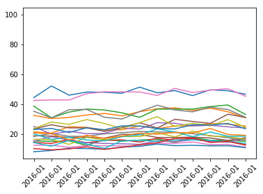
Save tidy data
Final step! I saved the tidy data as a CSV file and as a pickle file for future use in Python.
#### Save tidy dataos.chdir('C:\Users\Mushin Karim\Documents\Data\tidy_data\crimes_in_chicago')df.to_csv("tidy_py.csv", index=False)df.to_pickle("tidy.pk1")df.to_pickle("join.pk1")The tidy R CSV and the tidy Python CSV are not identical. Both contain the same number of rows (6,170,814). Both have the same number of columns with the same column names. However, the file sizes are different. The CSV from R is slightly bigger (1,415 MB versus Python’s 1,382 MB).
A visual inspection of the data in Excel revealed that the R CSV file listed “NA” for the “Latitude” and “Longitude” columns [4]. The rows are also sorted in different orders, but otherwise the tidy data CSV files appear similar.
Conclusion
The data wrangling steps described in this post depend on the given dataset. Another dataset may need additional steps. In my experience, different datasets encounter different errors after running the code, requiring a solution to get to the next step. Despite the differences between R and Python, I am more impressed with the similarities and pleased that the same data wrangling steps across the languages can produce near-identical tidy data.
We have wrangled the data and it is ready for analysis, visualisation and machine learning.
References and notes
- The maximum number of rows in an Excel worksheet is 1,048,576.
- Someone please point out a library that provides pain-free functions to create data types as datetimes.
- I made up these possible causes of duplicate entries for the same crime. In practice, I would investigate how crime events are logged into the system. I would be more than happy to visit Chicago to find out (low-crime Districts preferred).
- When opening the Python CSV file with Excel (I use Excel 2016) an error message appeared making reference to a “SYLK file format”. This is a known issue and is due to the first entry being “ID” (without quotations). The R CSV file has a leading quotation mark preventing the error. You can read about it here.

