
Welcome… To the fourth step of your Deep Learning adventure. Now, it’s time to continue with Self Organizing Maps or SOM’s. Sit back, relax, buckle up and get started with Self Organizing Maps (SOM’s)
Plan of Attack
Before we delve into this section on self-organizing maps (SOMs), let’s go through the section’s plan of attack. Here’s what you will get to learn in this section:
As with artificial neural networks, this part of the SOM section will give you a better understanding of what the sections aims at. This will happen as we examine together how the SOMs themselves learn.
We’ll have a recap of the process of K-means clustering which you have supposedly passed by during our machine learning course. Understanding K-means clustering will give you a more vivid comprehension of SOMs.
This question will be answered over two parts of this section. That’s not because of its complexity. Self-organizing maps are actually one of the simplest topics that we’ll cover in our course. It’s quite an interesting topic, though, and the material available for it is pretty rich.
Although the example we’ll be having in this section is very straightforward, it will reveal to you a lot about SOMs; how they work, structure themselves, learn, capture similarities and correlations in your data sets, and portrays them in a two-dimensional map.
Basically, it will wrap up everything that we’ll be covering in this section.
That’s the final part in the SOM section. We’ll have multiple SOMs on the screen in front of us, and you’ll learn how to read these maps, as well as various implementations of SOMs that will enable you to dig deeper into the topic if you happen to find it intriguing.
How do Self-Organizing Maps Work?
Now it’s time for our first tutorial on self-organizing maps (SOMs). You’ll find it to be surprisingly simple, although not without its intricacies. Clear your mind and let’s get to it.
We’ve already covered the three machine learning methods that fall into the category of “supervised deep learning.” These are:
- Artificial Neural Networks
- Convolutional Neural Networks
- Recurrent Neural Networks
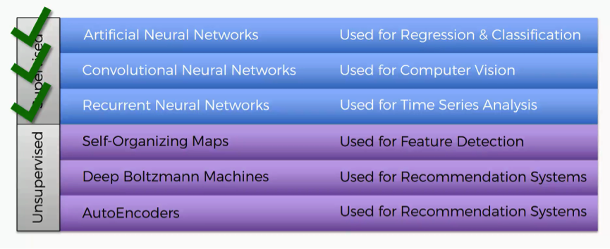
SOMs will be our first step into the unsupervised category. Self-organizing maps go back to the 1980s, and the credit for introducing them goes to Teuvo Kohonen, the man you see in the picture below. Self-organizing maps are even often referred to as Kohonen maps.

What is the core purpose of SOMs?
The short answer would be reducing dimensionality. The example below of a SOM comes from a paper discussing an amazingly interesting application of self-organizing maps in astronomy.
The example shows a complex data set consisting of a massive amount of columns and dimensions and demonstrates how that data set’s dimensionality can be reduced.
So, instead of having to deal with hundreds of rows and columns (because who would want that!), the data is processed into a simplified map; that’s what we call a self-organizing map. The map provides you with a two-dimensional representation of the exact same data set; one that is easier to read.
What exactly is the outcome to be gained from this process?
What you see below is an actual SOM. This map represents the levels of economic wellbeing across a wide range of countries.
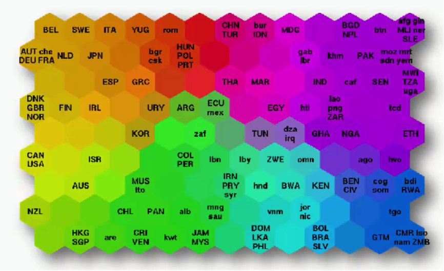
As you can see, the countries are lined up in a cluster, and their order inside that cluster is based on various indicators (e.g. health conditions, quality of education, average income per capita, etc.).
You can imagine this data set of 200+ countries to have started off with 39 different columns. It’s tough to imagine such a bulk of data, isn’t it?
That’s exactly why we use SOMs.
Instead of presenting you with each indicator separately, the SOM lines up the countries inside this cluster to make up a spectrum of wellbeing.
You can see the countries on the left side being the ones with the best economic statuses, although they vary in colors based on their positions within the category of high-income countries.
Then as you move to the right, you find the countries getting poorer until you reach the far right which contains the countries with the direst levels of poverty.
There’s an important difference between SOMs as an unsupervised deep learning tool and the supervised deep learning methods like convolutional neural networks that you need to understand.
While in supervised methods the network is given a labeled data set that helps it classify the data into these categories, SOMs receive unlabeled data. The SOM is given the data set and it has to learn how to classify its components on its own.
In this example, it would look at, say, Norway, Sweden, and Belgium, and left to its own devices, it learns that these countries belong together within the same area on the spectrum.
Besides giving us an easy way to read this data, SOMs have a wider range of uses.
For instance, you probably saw a map similar to the one below where countries are colored based on their human development scores, crime levels, military spending, etc.
Such maps can be colored using a SOM, since we can take the colors that the SOM chose for each group and apply it to our world map.
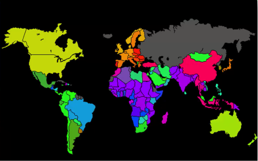
Here’s how the process goes:
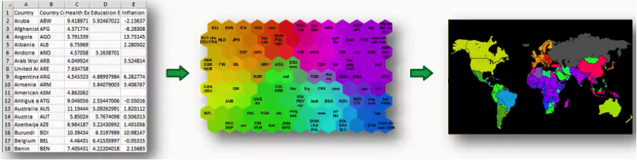
In this case, we got the data set from the World Bank containing all 39 indicators of human development, processed them into a SOM, and then applied that to a world map. As simple as that!
If you want to study this process at a more detailed level, we would recommend a paper titled “The Self-Organizing Map” that was authored by Tuevo Koheonen himself back in 1990. Now, off to the next tutorial!
Why revisit K-Means?
This tutorial is very brief as you can see. The only purpose of this tutorial is to discuss why we need to revisit K-means as we delve deeper into SOMs.
We discussed K-means before in one of our previous machine learning courses. Our next tutorial in this section will be based on a video taken from that course.
That tutorial will be an introduction to K-mean clustering to those of you who haven’t taken the course and memory refreshment for those who have. Learning about K-mean clustering will be extremely helpful when dealing with self-organizing maps. It’s not a major part of SOMs, but it will prepare you to understand them properly.
There are two major elements in K-means that will provide you with that introduction to both SOMs and unsupervised machine learning in general:
- You will get to see in the next video the push-and-pull movements that these nodes go through as they travel across the map. That process will give you a glimpse of what you will deal with when working with SOMs.
- Like SOMs, K-means are also unsupervised, although the K-means method is merely a machine learning algorithm rather than a neural network.
That’s it for this tutorial. You can now move on to the actual K-means tutorial.
K-Means Clustering (Refresher)
For starters, K-means is a clustering algorithm as apparent from the title of this tutorial. As we discuss K-means, you’ll get to realize how this algorithm can introduce you to categories in your datasets that you wouldn’t have been able to discover otherwise.
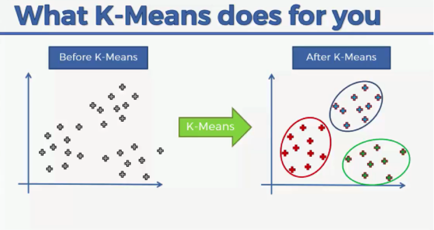
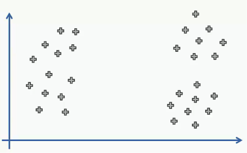
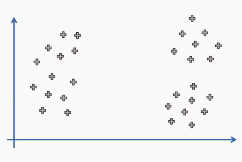
In this tutorial you’ll get to learn the K-means process at an intuitive level, and we’ll go through an example of how it works. Let’s get to it. The K-means process begins with a scatter plot like the one you see in the chart below.
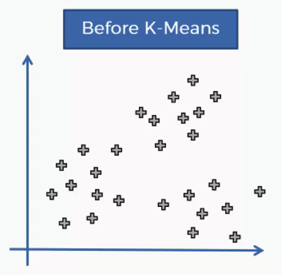
What this chart represents are two variables depicted on the X- and Y-axes, and the points represent our observations regarding these two variables.
The question is: How do we identify the categories using this data?
Should the observations be categorized by proximity, alignment or otherwise? How many categories are there?
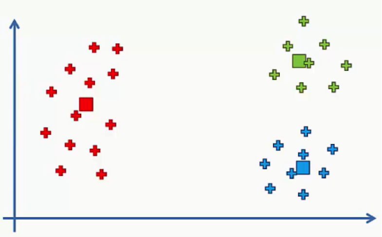
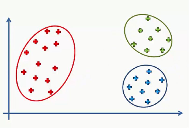
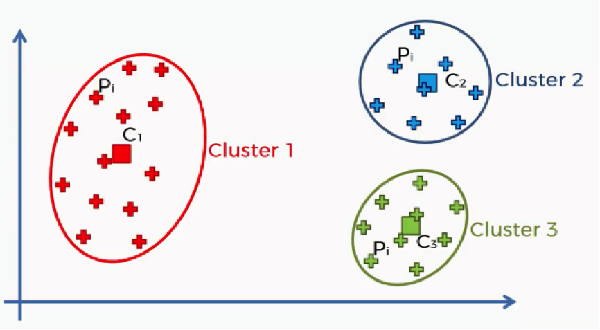
That’s where the K-means algorithm comes into play. It helps us identify the categories more easily as you can see in the image below.
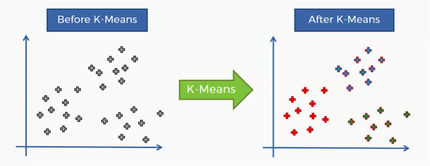
In this case we have three clusters.
Bear in mind that our example shows a two-dimensional dataset, and so it is only for purposes of illustration since K-means can deal with multidimensional datasets.
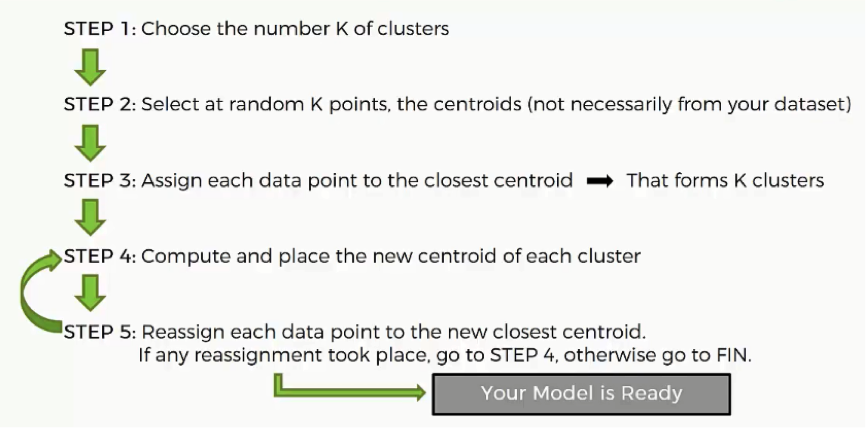
How does the K-means method work step by step?
- Step One: Choose the number of clusters.
Before processing the dataset into categories, the number of clusters has to be agreed upon.
- Step Two: Randomly select K points to act as centroids.
If you have a scatter plot like the one we examined earlier, all you need to do is choose a random (x,y) point. It doesn’t necessarily have to be one of the observation plots from your dataset.
Literally, any x-y value would do.
The most important thing is that you need as many centroids as clusters.
- Step Three: Assign each data point to the centroid closest to it.
This is how you actually form K clusters. As the data points are assigned to their centroids, the clusters emerge around these centroids.
To avoid any confusion, we’ll use Euclidean distance in our tutorials.
- Step Four: Compute and place the new centroid of each cluster.
You’ll see how this step is implemented when we get to the example.
- Step Five: Reassign the data points to the centroid that is closest to them now.
If any reassignments actually occur, then you need to go back to step 4 and repeat until there are no more to be made.
If there aren’t any, then that means that you’re done with the process and your model is ready.
This might be sounding a bit complex if it’s your first time to encounter K-means, but as we go through our visual example, you’ll see for yourself how simple the process can actually be.
Afterward, you’ll be able to refer to this 5-step manual whenever you’re dealing with K-means clustering.
A Two-Dimensional Example
In our example, we’ll be demonstrating each step separately.
Let’s go.
- Step One: Choose the number of Clusters
As we said earlier, you start off the K-means clustering process with a scatter plot chart like this one:
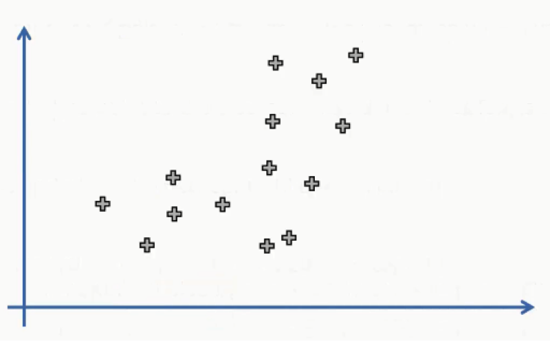
We have our observations plotted along the two-axes, each of which represents a variable.
You can see how tough it might be to categorize this dataset despite the fact that it’s merely a two-dimensional set. Imagine the difficulty of trying to do so with a multidimensional dataset. If it’s a 5-dimensional set, for instance, we wouldn’t even be able to display it in a scatter plot to begin with.
We’ll resort to the K-means algorithm to do the job for us, but in this example, we’ll be manually performing the algorithm. Usually, the algorithm is enacted using programming tools like Python and R.
For the sake of simplifying our example, we’ll agree on 2 as the number of our clusters. That means that K=2. Further down in this section, we’ll learn how to find the optimal number of clusters.
- Step Two: Randomly select K points to act as centroids.
In this step we can use one of the data points on the scatter plot or any other point.
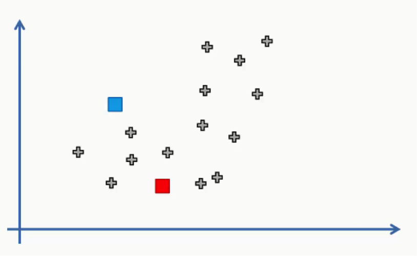
In this case, we didn’t use any of the data points as centroids.
- Step Three: Assign each data point to the centroid closest to it.
Now all we need to do is see which of these centroids is closest to each of our data points. Instead of doing that point by point, we’ll use a trick that you probably remember if you were awake during your high school geometry classes.
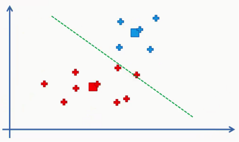
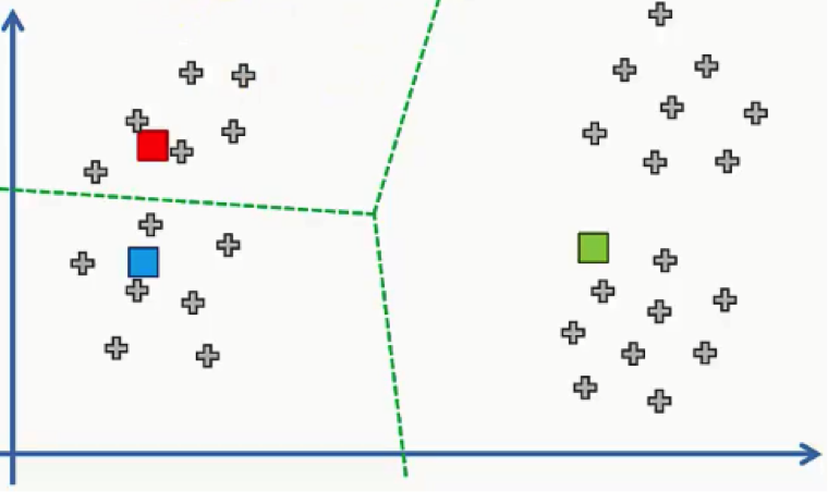
We’ll draw a straight line between the two centroids, then a perpendicular line right at the middle of this straight line. That’s what we will end up with:
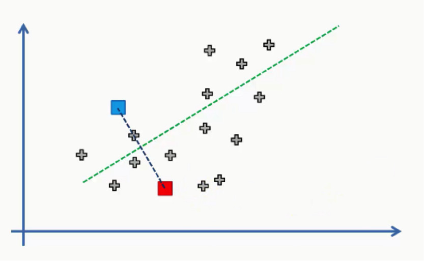
As we can see from the figure above, any data point falling above the green line is closer to the blue centroid, whereas any point beneath it is closer to the red one. We then color our data points by the colors of their centroids.
Just to remind you, we are using Euclidean distances here. There are various other methods for measuring distance, and it’s your job as a data scientist to find the optimal method for each case.
The reason we’re using Euclidean distance here is that it is the most straightforward of all the other methods.
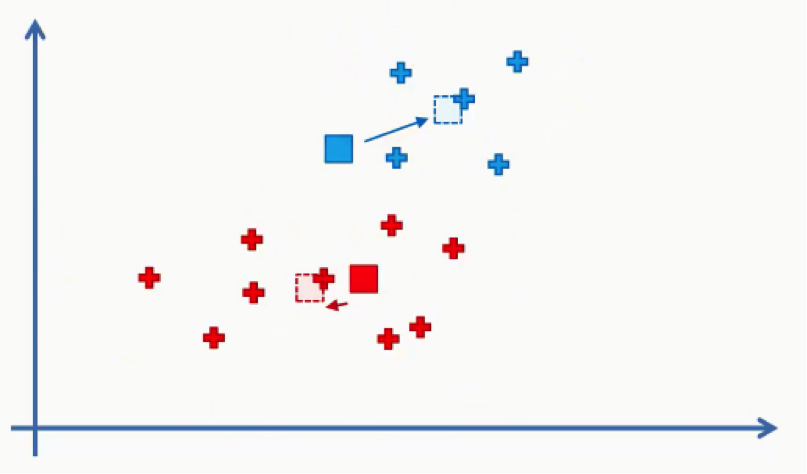
- Step Four: Compute and place the new centroid of each cluster.
Think of your centroids as weightless points with weighted data points gathered around them. We need to find and plot the new centroids at the center of each cluster’s mass like you see in the figure below.
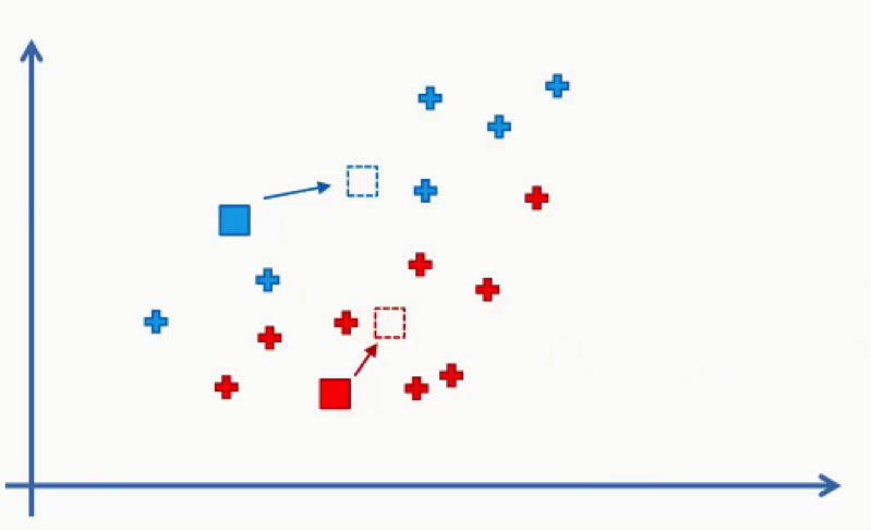
You can either intuitively find that center of gravity for each cluster using your own eyes, or calculate the average of the x-y coordinates for all the points inside the cluster.
- Step Five: Reassign the data points to the centroid that is closest to them now.
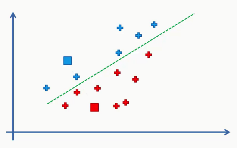
What we’ll do here is draw the same line that we drew in step three between our two new centroids.
As you can see, one of the red data points ended up in the blue cluster, and two blue points fell into the red cluster.
These points will be recolored to fit their new clusters. In this case, we’ll have to go back to step 4.
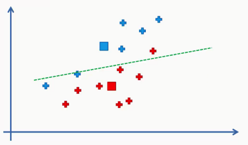
Then we will repeat step 5 by reassigning each data point to its new centroid.
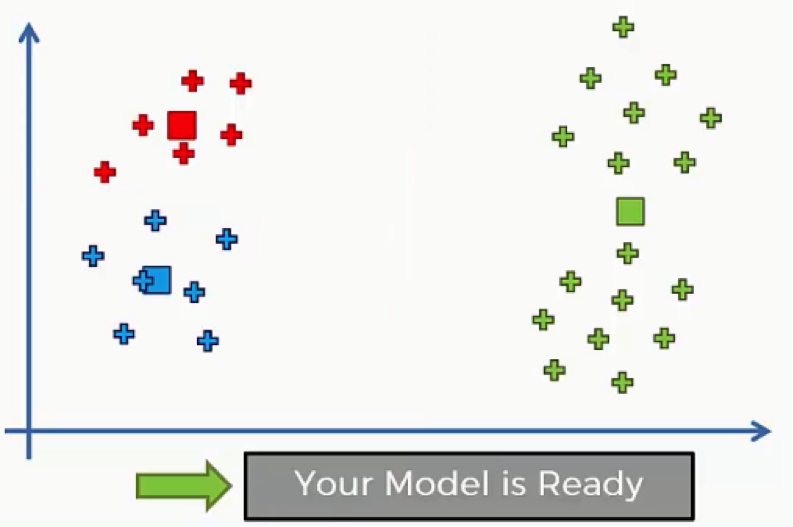
Again, we will end up with one red data point shifting to the blue cluster. This will take us back to step 4 and we’ll keep repeating until there are no more reassignments to be made. After a couple more repetitions of these steps, we’ll find ourselves with the figure below.
How do Self-Organizing Maps Learn? (Part 1)
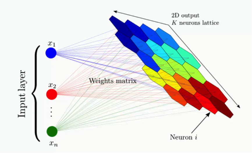
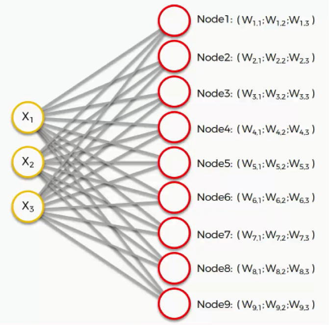
Now it’s time for us to learn how SOMs learn. Are you ready? Let’s begin. Right here we have a very basic self-organizing map.
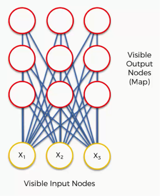
Our input vectors amount to three features, and we have nine output nodes.
If you remember the earlier tutorials in this section, we said that SOMs are aimed at reducing the dimensionality of your dataset.
That being said, it might confuse you to see how this example shows three input nodes producing nine output nodes. Don’t get puzzled by that. The three input nodes represent three columns (dimensions) in the dataset, but each of these columns can contain thousands of rows. The output nodes in an SOM are always two-dimensional.
Now what we’ll do is turn this SOM into an input set that would be more familiar to you from when we discussed the supervised machine learning methods (artificial, convolutional, and recurrent neural networks) in earlier sections.
Here’s what it would look like.
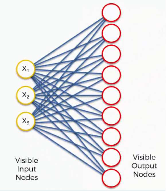
It’s still the exact same network yet with different positioning of the nodes. It contains the same connections between the input and the output nodes.
There are, however, differences in the SOMs from what we learned about the supervised types of neural networks:
- SOMs are much simpler.
- Because of their being different, some of the terms and concepts (e.g. weights, synapses, etc.) that we learned in earlier sections will carry different meanings in the context of SOMs. Try not to get confused by these terms.
Now, let’s take the topmost output node and focus on its connections with the input nodes. As you can see, there is a weight assigned to each of these connections.
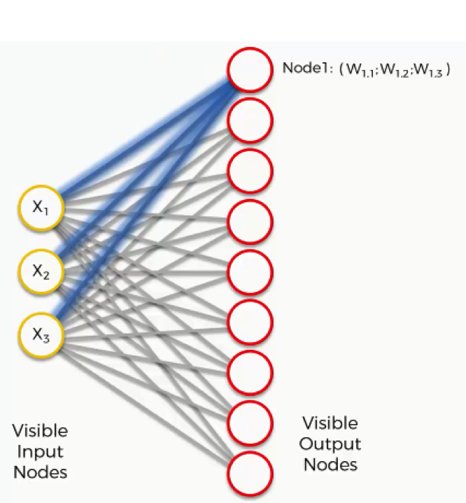
Again, the word “weight” here carries a whole other meaning than it did with artificial and convolutional neural networks.
For instance, with artificial neural networks we multiplied the input node’s value by the weight and, finally, applied an activation function. With SOMs, on the other hand, there is no activation function.
Weights are not separate from the nodes here. In an SOM, the weights belong to the output node itself. Instead of being the result of adding up the weights, the output node in an SOM contains the weights as its coordinates. Carrying these weights, it sneakily tries to find its way into the input space.
In this example, we have a 3D dataset, and each of the input nodes represents an x-coordinate. The SOM would compress these into a single output node that carries three weights.
If we happen to deal with a 20-dimensional dataset, the output node in this case would carry 20 weight coordinates.
Each of these output nodes do not exactly become parts of the input space, but try to integrate into it nevertheless, developing imaginary places for themselves.
The next step is to go through our dataset. For each of the rows in our dataset, we’ll try to find the node closest to it.
Say we take row number 1, and we extract its value for each of the three columns we have. We’ll then want to find which of our output nodes is closest to that row.
To do that, we’ll use the following equation.
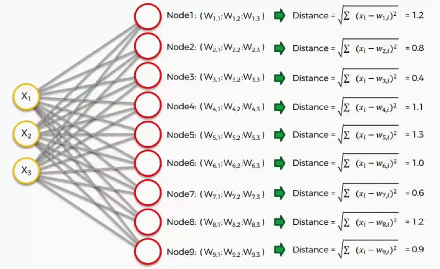
As we can see, node number 3 is the closest with a distance of 0.4. We will call this node our BMU (best-matching unit).
What happens next?
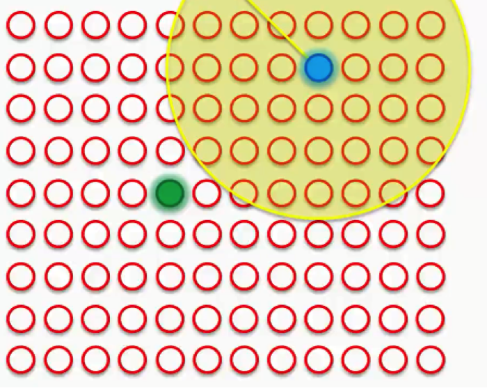
To understand this next part, we’ll need to use a larger SOM.
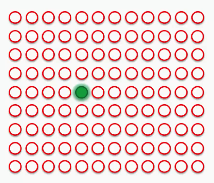
Supposedly you now understand what the difference is between weights in the SOM context as opposed to the one we were used to when dealing with supervised machine learning.
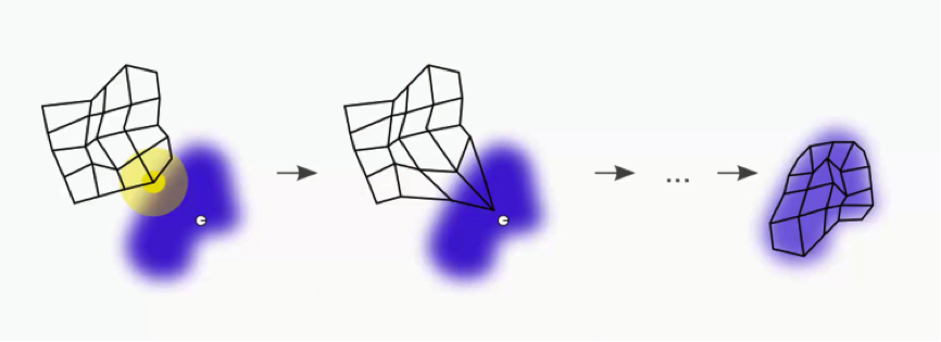
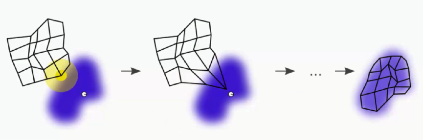
The green circle in the figure above represents this map’s BMU. Now, the new SOM will have to update its weights so that it is even closer to our dataset’s first row. The reason we need this is that our input nodes cannot be updated, whereas we have control over our output nodes.
In simple terms, our SOM is drawing closer to the data point by stretching the BMU towards it. The end goal is to have our map as aligned with the dataset as we see in the image on the far right.
That’s a long process, though. Right now we only care about that BMU. As you can see in the first image, the BMU (yellow circle) is the closest to the data point (the small white circle). As you can also see, as we drag the BMU closer to the data point, the nearby nodes are also pulled closer to that point.
Our next step would be to draw a radius around the BMU, and any node that falls into that radius would have its weight updated to have it pulled closer to the data point (row) that we have matched up with.
The closer a node is to the BMU, the heavier the weight that will be added to in its update.
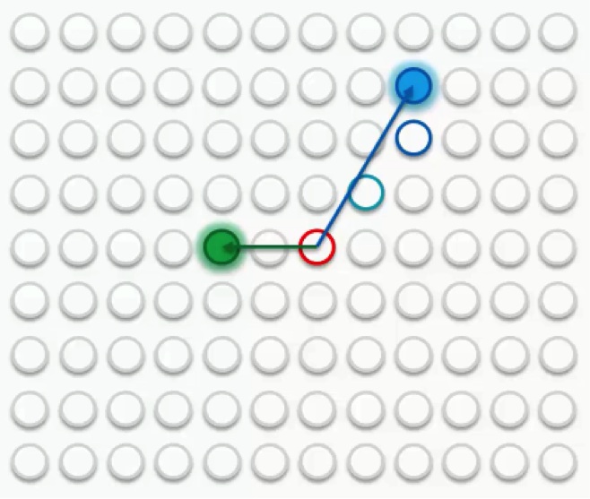
If we then choose another row to match up with, we’ll get a different BMU. We’ll then repeat the same process with that new BMU.
Sometimes a node will fall into both radii, the one drawn around the green BMU as well as the one around the blue BMU. In this case, the node will be affected more by its nearest BMU, although it would still be affected at a lesser degree by the further one.
If, however, the node is almost equidistant from both BMUs, its weight update would come from a combination of both forces.
This should clarify for you how a self-organizing map comes to actually organize itself. The process is quite simple as you can see. The trick is in its repetition over and over again until we reach a point where the output nodes completely match the dataset.
In the next tutorial, we’ll get to see what happens when a more complex output set with more BMUs has to go through that same process. We’ll see you in the next tutorial!
How do Self-Organizing Maps Learn? (Part 2)
Let’s move to the second part of our tutorial on how SOMs learn. Like we said at the end of our last tutorial, this time we’ll be examining the SOM learning process at a more sophisticated level.
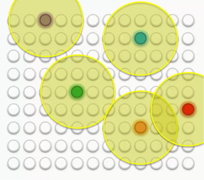
Our map this time will contain multiple best-matching units (BMUs) instead of just two.
We mentioned in our last tutorial how the BMUs will have to have their weights updated in order to be drawn closer to the data points.
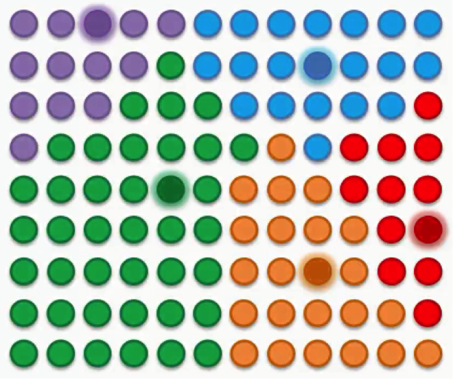
Then each of these BMUs will be assigned a radius like in the image below.
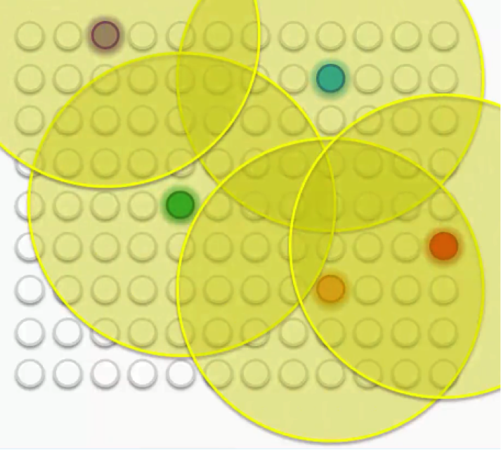
Let’s examine these BMUs one by one. Take the purple node at the top-left. It has been updated so as to be brought closer to the row with which it matches up. The other nodes that fall into its radius undergo the same updates so that they’re dragged along with it.
The same goes for each of the other BMUs along with the nodes in their peripheries.
Of course, in that process, the peripheral nodes are going through some push and pull since many of them fall within the radii of more than one BMU. They are updated by the combine forces of these BMUs, with the nearest BMU being the most influential.
As we repeat this process going forward, the radius for each BMU shrinks. That’s a unique feature of the Kohonen algorithm.
That means that each BMU will start exerting pressure on fewer nodes.
As we proceed, we move from trying to merely let our BMUs touch the data points to trying to align the entire map with the dataset with more precision.
In visual terms, that would lead us to a map that looks something like this:
After all the push and pull between the nodes and the different BMUs, we have come to a point where each node has been assigned a BMU.
There are a few points to bear in mind here:
- SOMs retain the interrelations and structure of the input dataset.
The SOM goes through this whole process precisely to get as close as possible to the dataset. In order to do that, it has to adopt the dataset’s topology.
- SOMs uncover correlations that wouldn’t be otherwise easily identifiable.
If you have a dataset with hundreds or thousands of columns, it would be virtually impossible to draw up the correlations between all of that data. SOMs handle this by analyzing the entire dataset and actually mapping it out for you to easily read.
- SOMs categorize data without the need for supervision.
As we mentioned in our introduction to the SOM section, self-organizing maps are an unsupervised form of deep learning. You do not need to provide your map with labels for the categories for it to classify the data.
It develops its own classes.
- SOMs do not require target vectors nor do they undergo a process of backpropagation.
If you remember from our artificial neural networks section, the network would need to be provided with a target vector (supervision). The data then goes through the network, extract results, compare them to the target vector, detect any errors, and then backpropagate these findings in order to update the weights.
Since we have no target vector, seeing as how SOMs are unsupervised, there would consequently be no errors for the map to backpropagate.
- There are lateral connections between output nodes.
The only connection that emerges between the output nodes in an SOM is the push-and-pull connection between the nodes and the BMUs based on the radius around each BMU.
There is no activation function as with artificial neural networks.
You will sometimes see the nodes lined up in a grid, but the only function for that grid is to clarify that these nodes are part of an SOM and to neatly organize them. The grid does not connect the nodes.
Additional Readings
If you’re interested in a slightly deeper introduction to SOMs, you can read this post from 2004 by Mat Buckland.
The post covers some of the math behind SOMs, which is quite straightforward compared to some of the mathematical operations that are used when dealing with neural networks.
He also breaks down in more detail the process by which nodes line up into the radii, how BMUs are drawn closer to the data points, etc. We’re now done with the theoretical part of the SOM section. In our next tutorial we’ll go together through a live example that demonstrates what we learned.
Live SOM example
Now we’re ready to look at a live example on SOMs. Although you’ll find it pretty simple and straightforward, this example will help you wrap your head around everything we discussed up until now in this section.
Two tutorials ago, we mentioned the website www.ai-junkie.com where we linked to a post on self-organizing maps. You’ll first need to visit this post on the website where you’ll find a zip file that we’ll be using in this example. Download the file and get ready to begin.
CAUTION: We are not affiliated with www.ai-junkie.com, so make sure you take the necessary precautions when operating this file.
The Example
The code in this file will create an SOM with input nodes represented by the eight colors below.
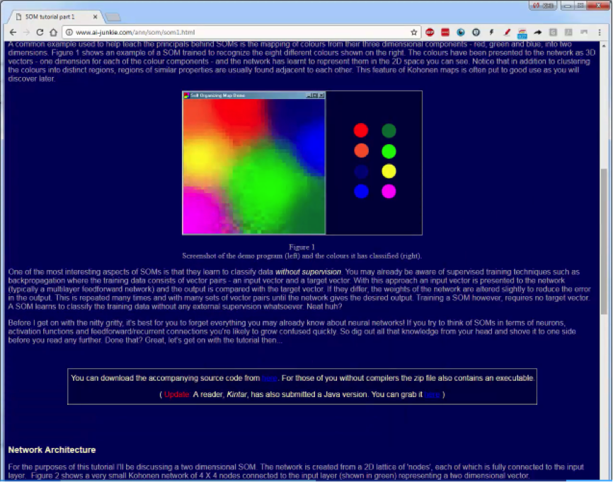
Each row in our dataset is represented by the RGB code of each color. We have, for example, the red color represented by (255,0,0), the orange at (255,165,0), and the blue at (0,0,255), etc.
Each of the eight colors represents a row, and each color carries three rows that are represented in the RGB code of that color. Once you open the file, the SOM in the below figure will appear. At the bottom-left side is the number of iterations, and you can press R in order to retrain the map.
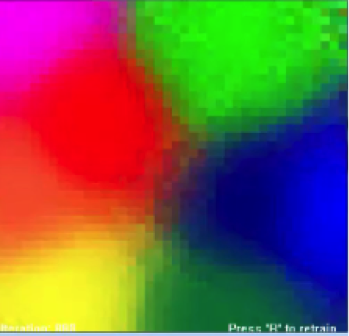
As you will see, every time you press R, the map will organize itself differently. Despite the changes, you will find that the map will preserve its correlations throughout every retraining step. That’s a brief example that you can experiment with on your own.
Besides the map itself, you’ll find the code to the SOM on the website with the file. You can take a look at how an SOM is coded and the logic on which it operates.
As you examine this material, you’ll notice how incredibly simple SOMs and the math behind them really are. That’s it for this tutorial. In our next tutorial, we’ll get to read SOMs at a more advanced level.
If you feel like you need a quick recap of the previous tutorials before getting to the next one, it would be best if you go through them briefly before moving on.
Reading an Advanced SOM
It’s now time to crank it up a notch and see what it takes to read a more advanced SOM then the ones we’ve been dealing with so far.
Here we have an example of an SOM that carries within it multiple SOMs.
Maps like this one will not always show up in your SOM-related projects, but it’s nevertheless a useful skill to know what to make of them.
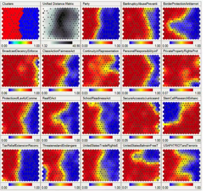
This SOM displays voting patterns inside the United States Congress, with each sub-SOM showing the patterns for a specific act or decision.
Without any supervision as usual, the SOM was able to monitor voting patterns among Congress members, and based on these patterns, it was able to divide the members into groups based on their partisan affiliations.
Let’s examine each SOM in that grid individually.
SOM 1×1: Clusters
There’s an interesting detail to take note of. Notice that the first SOM displaying the clusters actually differs from the “Party” SOM in the same row.
You would expect the clusters to be divided along partisan lines, but apparently, the SOM has detected some overlapping in the voting patterns of members from both parties.
The “Clusters” SOM is based on the sum of all the votes on all these different issues, and so it’s very likely to find members of the Democratic Party siding with the Republicans and vice versa.
SOM 1×2: Unified Distance Matrix
The Unified Distance Matrix, or the U-matrix, represents the distances between the points or nodes on the SOM.
The dark parts in that matrix represent the parts of the map where the nodes are far away from each other, and the lighter parts represent less distances between the nodes.
You can even notice that the darkest parts are the same parts where the clusters are divided, which logically are the parts with the widest distances between the nodes.
SOM 1×4: Bankruptcy/Abuse Prevention
In this map, you can see that the border between the two sides is drawn a bit further to the right from where it appears in the “Clusters” SOM. That means that more people took the Republican side, including members who appear on the Democratic Party’s side in the “Clusters” map.
SOMs make it possible for you to visually detect these deviations without having to monitor all the data.
SOM 1×5: Border Protection/Anti-Terrorism
A lot of members from the Republican cluster appear to have taken the Democratic side which interestingly deviates at the middle more than anywhere else.
SOM 1×6: Broadcast Decency Enforcement
What you see in this map is one of the rare incidents of cross-party unity in the US Congress. Almost the entire Democratic bloc appears to have turned conservative on that particular issue.
Now you probably get the idea of how to read an SOM of that kind. You will find that the simplicity of SOMs facilitates various forms of implementation. Observe this beautiful collage of confusing figures. These are all forms of SOMs.
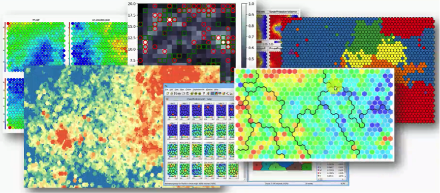
With enough of an intuitive ability to read an SOM, which this section is aimed at, you will find yourself capable of reading most of these despite their countless different forms.
Additional Reading
There is a particular SOM up there in the collage that you should check out and examine more closely. It’s this one below.
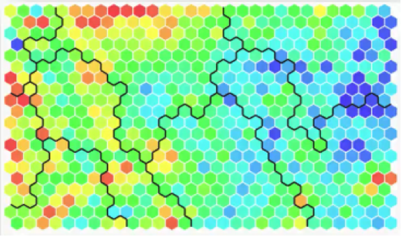
You will find it in an article from 2013 titled “SOM – Creating hexagonal heatmaps with D3.js” by Nadieh Bremer. The blogpost was posted on Visual Cinnamon.
As you can see from the name, the SOM was coded using D3.js. You will probably find it interesting to learn more about this amazingly useful JavaScript library.
Also, Nadieh Bremer, the author, made a great job of presenting the SOM in the blogpost. She shows how she came up with this visual representation, the hexagons, and displays the code for all of that. If you have any background in coding, you shouldn’t find difficulties at all in understanding the code.
You’ll find the full code if you visit this link.
If you’re interested in trying out D3.js, then while you’re on that website (bl.ocks.org) where the code is, check out the “Popular” section linked to over there at the top right corner.
You’ll find a goldmine of D3.js-based graphs and representations including SOMs. You’ll see how interactive D3.js can make things.
How to Boost Your Understanding of SOMs
The most important thing to walk away with from this tutorial, and from the section on SOMs as a whole, is that SOMs are by far the simplest type of neural network and form of visual data representation that we discussed.
You don’t need too much coding experience to be able to code an SOM using R, Python, JavaScript, Java, or pretty much any coding language out there.
It’s not exactly a complex job, especially given the fact that you’re not limited to any shapes, formats, or otherwise. You can use square, circles, hexagons, or whatever else you wish to use. The mathematics behind SOMs is also extremely uncomplicated.
All you need to do is find one programming language that you are absolutely comfortable with and challenge yourself at creating a few SOMs using different forms of implementation if possible.
You can search online for libraries that can give you the kick-start there.
The next two tutorials are extras. We’ll be having two more parts on K-means clustering. You don’t need to take these tutorials, but if you really want to get a tighter grasp on our original topic, you’ll absolutely find them helpful.
EXTRA: K-means Clustering (part 2)
This time we’ll focus on a very specific part of the K-means algorithm; the Random Initialization Trap. Let’s start right off the bat with an example that will demonstrate what the random initialization trap actually is.
Here’s a scatter plot with two variables (x and y).
Let’s say we’ve decided to divide our data points into three clusters.
Intuitively, you can probably look at that scatter plot and guess how the three clusters are going to be lined up and which group of data points will fall into each cluster.
After determining our centroids, assigning each centroid its data points, and performing the rest of the K-means algorithm, we would end up with the following three clusters.
The question here is whether we can change the results and end up with different clusters if we changed the positions of our centroids.
Of course, what we expect from this algorithm is to provide us with proper results, not ones that we can manipulate by playing around with the centroids. What if we had a bad random initialization? What happens then? In case you’re confused as to what defines a good or a bad random initialization, just know that we’re using the term “bad” in the loosest sense possible.
Let’s go through a quick recap of the K-means process.
As you can see, the entire process is dependent on the first two steps which you are responsible to arbitrarily decide. After you choose the centroids, the rest of the algorithm becomes more deterministic.
Now, let’s try to change our centroids in the second step and see how the rest of the algorithm will play out.
Here are our new centroids, and just to make things easier on ourselves, we can use the same equidistant lines that we used in part 1 on K-means clustering.
These lines will help us assign data points to their nearest centroids more efficiently.
We’ll then move on to step 4 where we compute and place the new centroids. This action is supposed to be done over and over again until there are no reassignments of data points to be made.
You can obviously see the difference between these clusters and the ones we had at the beginning of our example.
Random Initialization Trap
If you look at the clusters below, which were gathered around our original centroids, as we said earlier, you can intuitively detect the patterns before the assignment of the data points to centroids was actually made.
That’s the difference between the two situations. The new centroids with the clusters formed around them are not exactly “intuitively detectable.” You wouldn’t look at the scatter plot and imagine these as the clusters that you will end up with.
Here’s a prime example of how your initialization of the K-means operation can impact the results in a major way. That’s what is known as the Random Initialization Trap.
K-Means++
There’s a remedy for this problem that is used as a supplement to the K-means algorithm. It’s called the K-means++. We won’t discuss this algorithm or its structure in depth, but you only need to know for now that it is hugely beneficial in solving this initialization problem.
Here’s a link to the K-means++ page on Wikipedia. You can do some additional reading about the topic on your own. The good news is that you don’t need to implement the K-means++ algorithm yourself. Whether you’re using R or Python in the process, the K-means++ is implemented in the background.
You only need to make sure that you are using the right tools in creating your K-means clusters and the correction will be automatically taken care of.
It’s a useful thing to understand nevertheless. It helps you understand the fact that, despite the random selection, there is a specific “correct” cluster that you’re searching for, and that the other clusters that can emerge might be wrong.
They can at least be “undesirable.” That’s it for this part, and as we said, it can do you some good to read about K-means++ as an introduction to what goes on underneath the hood.
EXTRA: K-means Clustering (part 3)
So far we have tried out multiple examples on the K-means process and in the last tutorial we introduced K-means++ as a way to counter the random initialization trap.
In all these cases, we were working with predetermined numbers of clusters. The question that we’ll try to answer in this tutorial is: How do we decide the right number of clusters in the first place? There’s an algorithm that specifically performs this function for us, and that’s what we’ll be discussing here. Again, we’ll start right away with an example.
Here we have a scatter plot representing a dataset where we have two variables, x and y.
By applying the K-means algorithm to this dataset with the number of clusters predetermined at 3, we would end up with the following outcome.
Keep in mind that the K-means++ had to be implemented in order for us to avoid the Random Initialization Trap. As we mentioned in the previous tutorial, though, you do not need to concern yourself with how that happens at the moment.
Now we want to know the metric or the standard that we can refer to when trying to come up with the “right” number of clusters.
Are 3 clusters enough? Or are 2 just enough? Or perhaps we need 10 clusters? More importantly, what are the possible outcomes that each of these scenarios can leave us with? In comes the WCSS.
Within Cluster Sum of Squares (WCSS)

That might look a bit confusing to you, but there’s no need for panicking. It’s simpler than you think.
Here’s a quick breakdown of the WCSS. Each of the elements in this algorithm is concerned with a single cluster. Let’s take the first cluster.
What this equation signifies is this: For Cluster 1, we’ll take every point (Pi) that falls within the cluster, and calculate the distance between that point and the centroid (C1) for Cluster 1.
We then square these distances and, finally, calculate the sum of all the squared distances for that cluster. The same is done for all the other clusters. How does this help us in knowing what number of clusters we should use?
That’s our next point.
Let’s take an example that we previously discussed where we have a single cluster. We’ll see, roughly, what results that will give us when put through the WCSS algorithm and how that would change as we add more clusters.
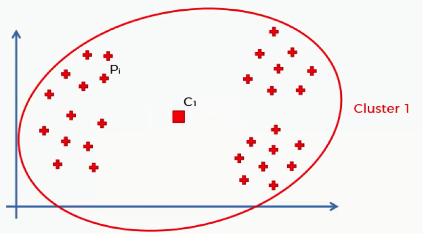
Of course, with that many data points inside a single cluster and given their wide distances from the cluster’s centroid, we’ll inevitably end up with a fairly large sum.
Let’s split up that same scatter plot into two clusters and see what happens.
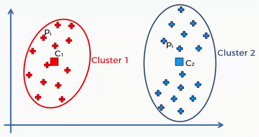
As you can see, now that we have more clusters, each data point will find itself nearer to its centroid. That way the distances, and consequently the sum of squared distances, will become smaller than when we had a single centroid.
Now, let’s step it up another cluster.
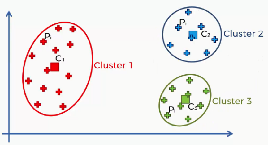
The cluster on the left did not change at all, and so the sum of its squared distances will remain unchanged as well.
The cluster that was on the right in the previous step has now been split up into two clusters, though. That means that each data point has moved even closer to its centroid.
That means that the overall sum will again decrease. Now that you get the idea, we can ask the question of “how far can our WCSS keep on decreasing?”
Our limit is to have one cluster for each data point. You just can’t have 21 clusters for 20 data points. You need each point to be matched up with one centroid.
You can now take a moment to think of what would happen to the WCSS results if we created a cluster for each point.
If you said to yourself that you would end up with ZERO then you are absolutely right.
If each point has its own centroid, then that means that the centroid will be exactly where the point is. That, in turn, would give us a zero distance between each data point and its centroid, and as we all (hopefully) know, the sum of many zeros is a zero.
As the WCSS decreases with every increase in the number of clusters, the data points become better fit for their clusters.
So, do we just keep working towards smaller WCSS results or is there a point before the zero level which we can consider optimal?
This next graph can help us answer this question.
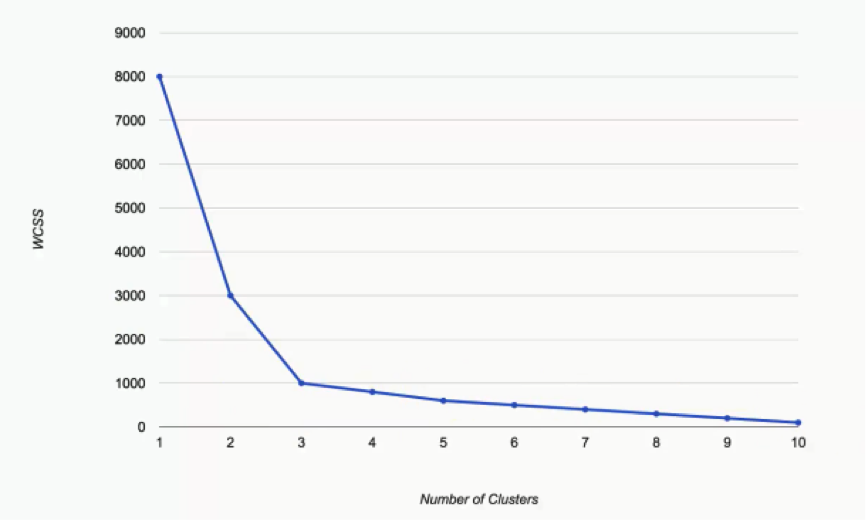
What we have here are the WCSS results as we incrementally increase the number of clusters in a dataset.
You can see that as we move from one cluster to two, the WCSS takes a massive fall from 8,000 to 3,000. It’s unimportant to think of the significance of these numbers at the moment. Let’s just focus on the degrees of change.
As we move from two to three, the WCSS still decreases substantially, from 3,000 to 1,000. From that point on, however, the changes become very minimal, with each cluster only shaving off 200 WCSS points or less. That’s our hint when it comes to choosing our optimal number of clusters. The keyword is: Elbow.
The Elbow Method
What is meant by the “Elbow Method” is looking for the point on this graph where the last substantial change has occurred and the remaining changes are insignificant. In this case, we reach that point at 3 clusters.
If you look at the curve at 3, you will see an elbow shape.
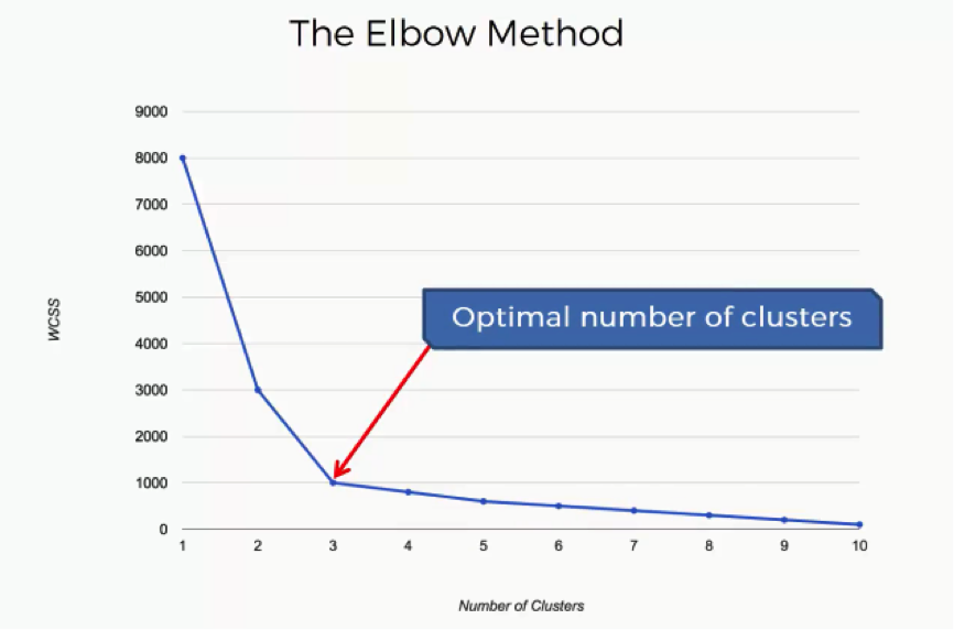
Of course, the “elbow” in your graph will not always be as obvious as in this example. You’re likely to have situations where each person would choose a different point, each thinking that theirs is the optimal point.
That’s where you have to make your judgment call as a data scientist. The Elbow Method can only give you a hint at where to look.
By now you have all the knowledge you need about K-means clustering to move on to the next step.
We’ve set up some exciting challenges that will give you all the practice you need to master K-means clustering using various languages.
Get ready to conquer this topic once and for all!