


Step 3 of your Deep Learning path: Recurrent Neural Networks. The arbitrary length brother of Convolutional Neural Networks. But you already knew that… right? If not, don’t worry!
The Ultimate Guide to Recurrent Neural Networks is here! This guide will help you master Recurrent Neural Networks and you’ll be able to visit it recurrently 🙂 (pun intended). Ready or not, here we go!
Plan of Attack
Are you excited about the idea to uncover the essence of Recurrent Neural Networks?
Hope you are… because we are now venturing into a complex, very forward-looking and cutting-edge areas of deep learning!
But what’s really important to keep in mind – this going to be very, very fun! So, how are we going to approach this section in Deep Learning?
First of all, we will learn the idea behind how Recurrent Neural Networks work and how they compare to the human brain.
Then, we’ll talk about the Vanishing Gradient Problem – something that used to be a major roadblock in the development and utilization of RNN.
Next, we’ll move on to the solution of this problem – Long Short-Term Memory (LSTM) neural networks and their architecture. We’ll break down the complex structure inside these networks into simple terms and you’ll get a pretty solid understanding of LSTMs.
Then, we’ll have a look at some great practical examples to get an idea on what’s actually going on in the brain of LSTM.
Finally, we will have an extra tutorial on LSTM variations just to get you up to speed on what other options of LSTM exist out there in the world.
Ready to get started?
Then move on to our next section!
The Idea Behind Recurrent Neural Networks
Recurrent Neural Networks represent one of the most advanced algorithms that exist in the world of supervised deep learning. And you are going to grasp it right away. Let’s get started!
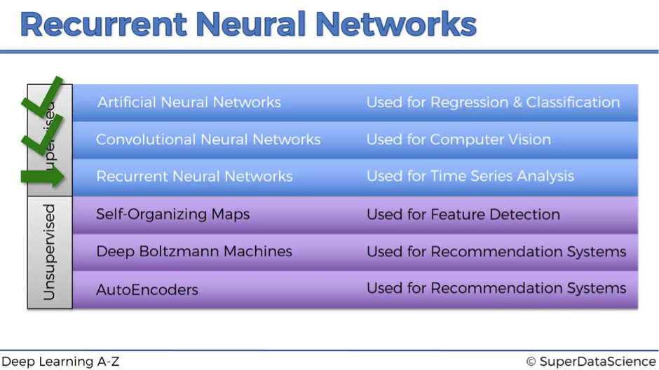
Here is our low breakdown of supervised vs. unsupervised deep learning branches:
- We’ve already talked about Artificial Neural Networks (ANN) and Convolutional Neural Networks (CNN).
- And now we’re starting to discover the idea behind Recurrent Neural Networks (RNN).
Neural Networks and Human Brain
As you might know already, the whole concept behind deep learning is to try to mimic the human brain and leverage the things that evolution has already developed for us.
So, why not to link different algorithms that we’ve already discussed to certain parts of the human brain?
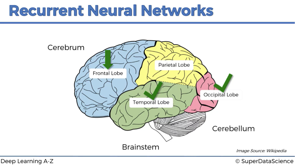
The human brain has got 3 parts: cerebrum, which is all of these colored parts on the image below, cerebellum, or “little brain” in Latin, and brainstem, which connects the brain to the organs. Then, the cerebrum has 4 lobes:
- temporal lobe,
- frontal lobe,
- occipital lobe,
- parietal lobe.
Temporal lobe and ann
The temporal lobe might be well linked to the ANN with its main contribution – the weights.
The fact that ANN can learn through prior experience, prior epochs and prior observations – that’s extremely valuable.
Weights represent long-term memory: ones you’ve run your ANN and you’ve trained it, you can switch it off and come back later because with the known weights the network will process the input the same way as it would yesterday and as it will tomorrow.
Of course, weights exist across the whole brain, but philosophically ANNs are a start to deep learning, and so we can say that they represent the long-term memory, which the temporal lobe of the human brain also does.
Occipital lobe and cnn
Next, we’re going to link the occipital lobe to CNN. As we already know, CNNs are responsible for computer vision, recognition of images and objects, which makes them a perfect link to the occipital lobe.
Frontal lobe and rnn
RNNs are like short-term memory. You will learn that they can remember things that just happen in a previous couple of observations and apply that knowledge in the going forward. For humans, short-term memory is one of the frontal lobe’s functions.
That’s why we are going to link RNNs to this lobe of the human brain.
Parietal lobe and …
The parietal lobe is responsible for sensation, perception and constructing a spatial-coordination system to represent the world around us, and we are yet to create a neural network which will fit into this category.
Now let’s move from neuroscience to our favorite neural networks.
Representation of the Recurrent Neural Networks
We begin with a transformation of a simple ANN showed below into RNN.
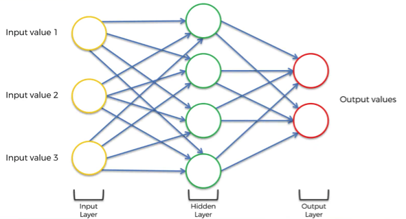
This takes 5 steps:
- Squashing the network. The layers are still there but think of it as if we’re looking from underneath this neural network.
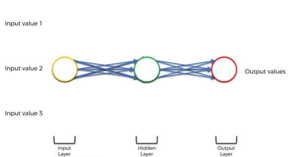
- Changing the multiple arrows into two.
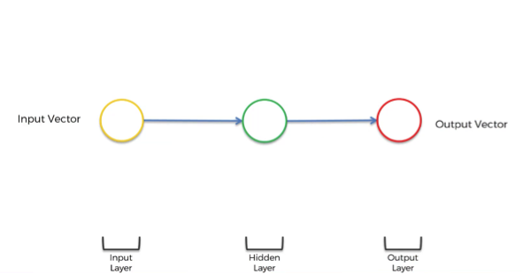
- Twisting it to make it vertical because that’s the standard representation.
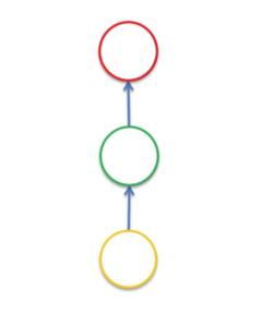
- Adding a line, which represents a temporal loop. This is an old-school representation of RNNs and basically means that this hidden layer not only gives an output but also feeds back into itself.
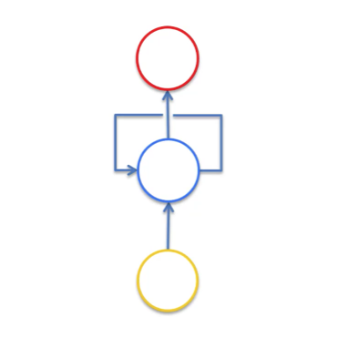
- Unrolling the temporal loop and representing RNNs in a new way. Now each circle represents not only one neuron, but a whole layer of neurons.
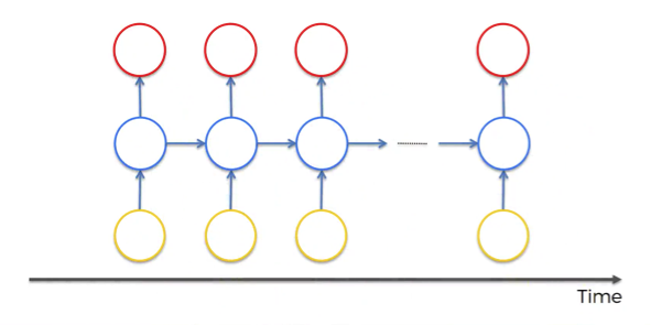
So, we’ve got inputs, hidden layer and outputs as usually but now the neurons are also connected to themselves through time.
The idea behind RNNs is that the neurons have some sort of short-term memory providing them with the possibility to remember, what was in this neuron just previously. Thus, the neurons can pass information on to themselves in the future and analyze things.
That’s kind of like when you’re reading this article – it would be really sad if you couldn’t remember what was in the previous paragraph or sentence. Now as you do remember those things, you can understand what we’re talking about in the current section.
Why would we deprive artificial construct, which is supposed to be a syntactic human brain, of something so powerful as a short-term memory?
And that’s where Recurrent Neural Networks come in.
Examples of RNN Application
One to many This is a network with one input and multiple outputs.
For instance, it could be an image (input), which is described by a computer with words (outputs). You can see such example in the image below.
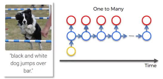
This picture of the dog first went through CNN and then was fed into RNN. The network describes the given picture as “black and white dog jumps over bar”. This is pretty accurate, isn’t it?
While CNN is responsible here for image processing and feature recognition, our RNN allows the computer to make sense out of the sentence. As you can see, the sentence actually flows quite well.
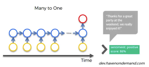
Many to one
An example of this relationship would be sentiment analysis, when you have lots of text, such as a customer’s comment, for example, and you need to gauge what’s the chance that this comment is positive, or how positive this comment actually is, or how negative it is.
Many to many
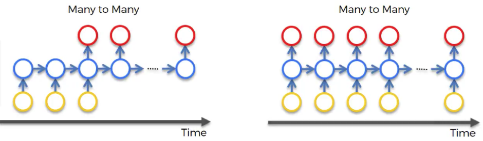
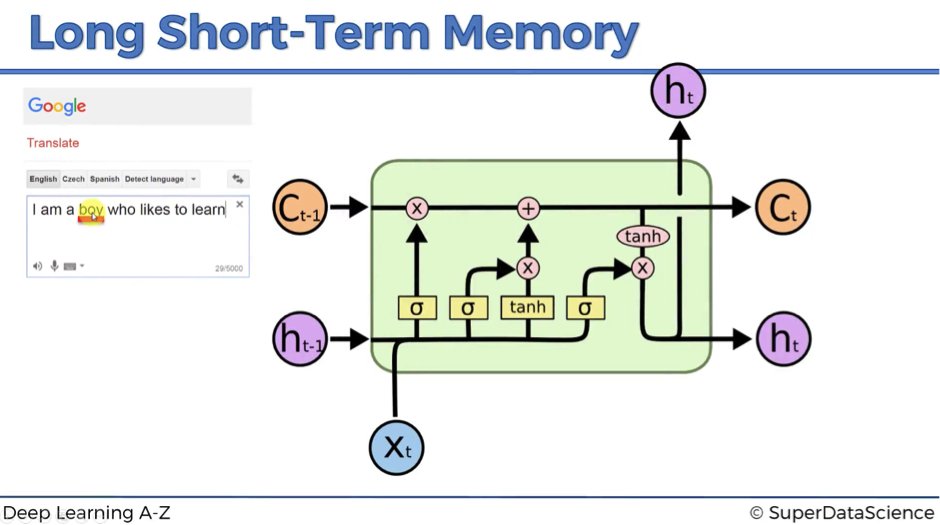
Translations can be a good example of many to many type of network. Let’s have a look at a particular instance from Google Translator. We don’t know if Google Translator uses RNNs or not, but the concept remains the same.
As you can see in the picture below, we’re translating one sentence from English to Czech. In some other languages, including Czech, it is important for the verb phrase, what gender your person is.
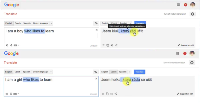
So, when we have “a boy” in the input sentence, the translation of the “who likes” part looks like “který rád”. But as we change a person to “a girl”, this part changes to “která ráda”, reflecting the change of the subject.
The concept is the following: you need the short-term information about the previous word to translate the next word.
You can’t just translate word by word. And that’s where RNNs have power because they have a short-term memory and they can do these things.
Of course, not every example has to be related to text or images. There can be lots and lots of different applications of RNN.
For instance, many to many relationship is reflected in the network used to generate subtitles for movies. That’s something you can’t do with CNN because you need context about what happened previously to understand what’s happening now, and you need this short-term memory embedded in RNNs.
Additional Reading
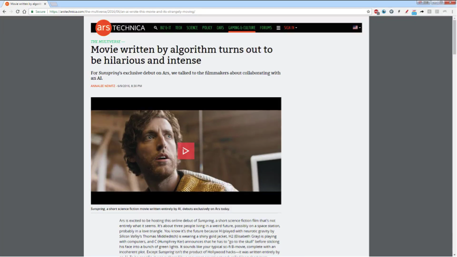
Actually, we are going to have additional watching instead of additional reading for this particular topic. Please check this movie, called Sunspring (2016).
Some exciting facts about the movie:
- It was entirely written by Benjamin, who is an RNN – or LSTM to be specific.
- The movie is only 9 minutes long and it’s really fun.
- You’ll notice that Benjamin is able to construct sentences, which kind of make sense for the most part.
- However, Benjamin still lacks a bigger picture and cannot come up with a plot that constantly makes sense. This will be probably the next step for RNNs.
The technology is only peaking up recently and maybe if you’re reading this article 5 years from now, you are laughing and thinking that you’ve already passed this milestone.
So, that’s what RNNs are in a nutshell. Move on to the next article to dig deeper.
The Vanishing Gradient Problem
Today we’re going to jump into a huge problem that exists with RNNs.But fear not!
First of all, it will be clearly explained without digging too deep into the mathematical terms.
And what’s even more important – we will discuss the solution to this problem in our next article from the deep learning series.
So, what is this problem called vanishing gradient?
People Behind Recurrent Neural Networks
The problem of the vanishing gradient was first discovered by Sepp (Joseph) Hochreiter back in 1991. Sepp is a genius scientist and one of the founding people, who contributed significantly to the way that we use RNNs and LSTMs today.
The second person is Yoshua Bengio, a professor at the University of Montreal.
He also discovered the vanishing descent problem but a bit later – he wrote about it in 1994. Yoshua is another person pushing the envelope in the space of deep learning and RNNs, in particular.
If you check his profile at the University of Montreal, you will find that he has contributed to over 500 research papers!
This is just to give you a quick idea, who are these people behind the RNN advancements.
Now, let’s proceed to the vanishing gradient problem itself.
Explaining the Vanishing Gradient Problem
As you remember, the gradient descent algorithm finds the global minimum of the cost function that is going to be an optimal setup for the network.
As you might also recall, information travels through the neural network from input neurons to the output neurons, while the error is calculated and propagated back through the network to update the weights.
It works quite similarly for RNNs, but here we’ve got a little bit more going on.
- Firstly, information travels through time in RNNs, which means that information from previous time points is used as input for the next time points.
- Secondly, you can calculate the cost function, or your error, at each time point.
Basically, during the training, your cost function compares your outcomes (red circles on the image below) to your desired output.
As a result, you have these values throughout the time series, for every single one of these red circles.
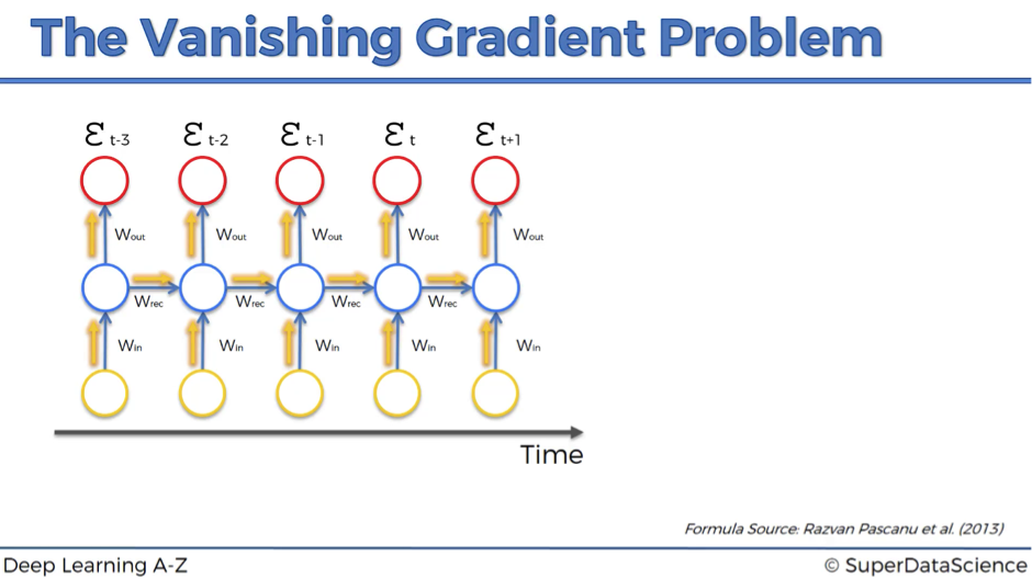
Let’s focus on one error term et.
You’ve calculated the cost function et, and now you want to propagate your cost function back through the network because you need to update the weights.
Essentially, every single neuron that participated in the calculation of the output, associated with this cost function, should have its weight updated in order to minimize that error. And the thing with RNNs is that it’s not just the neurons directly below this output layer that contributed but all of the neurons far back in time. So, you have to propagate all the way back through time to these neurons.
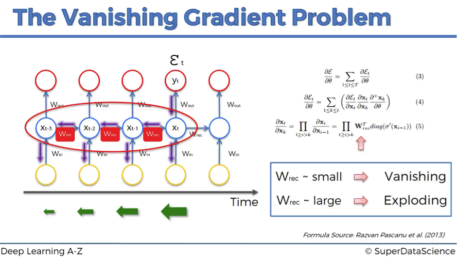
The problem relates to updating wrec (weight recurring) – the weight that is used to connect the hidden layers to themselves in the unrolled temporal loop.
For instance, to get from xt-3 to xt-2 we multiply xt-3 by wrec. Then, to get from xt-2 to xt-1 we again multiply xt-2 by wrec. So, we multiply with the same exact weight multiple times, and this is where the problem arises: when you multiply something by a small number, your value decreases very quickly.
As we know, weights are assigned at the start of the neural network with the random values, which are close to zero, and from there the network trains them up. But, when you start with wrec close to zero and multiply xt, xt-1, xt-2, xt-3, … by this value, your gradient becomes less and less with each multiplication.
What does this mean for the network?
The lower the gradient is, the harder it is for the network to update the weights and the longer it takes to get to the final result.
For instance, 1000 epochs might be enough to get the final weight for the time point t, but insufficient for training the weights for the time point t-3 due to a very low gradient at this point.
However, the problem is not only that half of the network is not trained properly.
The output of the earlier layers is used as the input for the further layers. Thus, the training for the time point t is happening all along based on inputs that are coming from untrained layers. So, because of the vanishing gradient, the whole network is not being trained properly.
To sum up, if wrec is small, you have vanishing gradient problem, and if wrec is large, you have exploding gradient problem.
For the vanishing gradient problem, the further you go through the network, the lower your gradient is and the harder it is to train the weights, which has a domino effect on all of the further weights throughout the network.
That was the main roadblock to using Recurrent Neural Networks.
But let’s now check what are the possible solutions to this problem.
Solutions to the Vanishing Gradient Problem
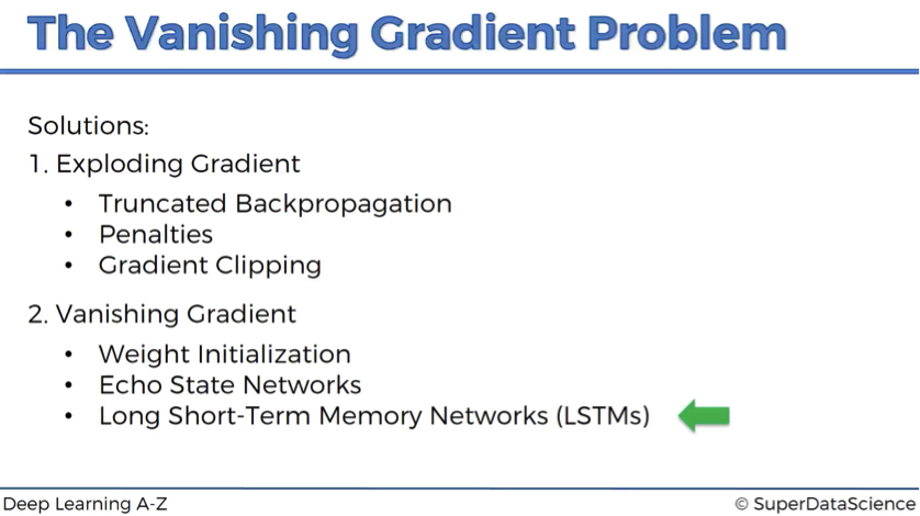
In case of exploding gradient, you can:
- stop backpropagating after a certain point, which is usually not optimal because not all of the weights get updated;
- penalize or artificially reduce gradient;
- put a maximum limit on a gradient.
In case of vanishing gradient, you can:
- initialize weights so that the potential for vanishing gradient is minimized;
- have Echo State Networks that are designed to solve the vanishing gradient problem;
- have Long Short-Term Memory Networks (LSTMs).
LSTMs are considered to be the go-to network for implementing RNNs, and we’re going to discuss this solution in depth in our next article.
Additional Reading
You can definitely reference the original works of the most significant contributors to this topic:
- Untersuchungen zu dynamischen neuronalen Netzen by Sepp (Joseph) Hochreiter (1991). Please note that it is completely in German.
- Learning long-term dependencies with gradient descent is difficult by Yoshua Bengio et al. (1994).
We also recommend looking into the following paper, which is quite recent and by the way, has got Yoshua Bengio as a co-author:
- On the difficulty of training recurrent neural networks by Razvan Pascanu et al. (2013).
That was the vanishing gradient problem. Can’t wait to know the solution to this fundamental problem? Then move on to our next article on the Long Short-Term Memory Networks.
Long Short Term Memory – (LSTM)
Long short-term memory (LSTM) network is the most popular solution to the vanishing gradient problem.
Are you ready to learn how we can elegantly remove the major roadblock to the use of Recurrent Neural Networks (RNNs)?
Here is our plan of attack for this challenging deep learning topic:
- First of all, we are going to look at a bit of history: what LSTM came from, what was the main idea behind it, why people invented it.
- Then, we will present the LSTM architecture.
- And finally, we’re going to have an example walkthrough.
Let’s get started!
Refresh on the Vanishing Gradient Problem
LSTMs were created to deal with the vanishing gradient problem. So, let’s have a brief reminder on this issue.
As we propagate the error through the network, it has to go through the unraveled temporal loop – the hidden layers connected to themselves in time by the means of weights wrec.
Because this weight is applied many-many times on top of itself, that causes the gradient to decline rapidly.
As a result, weights of the layers on the very far left are updated much slower than the weights of the layers on the far right.
This creates a domino effect because the weights of the far-left layers define the inputs to the far-right layers.
Therefore, the whole training of the network suffers, and that is called the problem of the vanishing gradient.
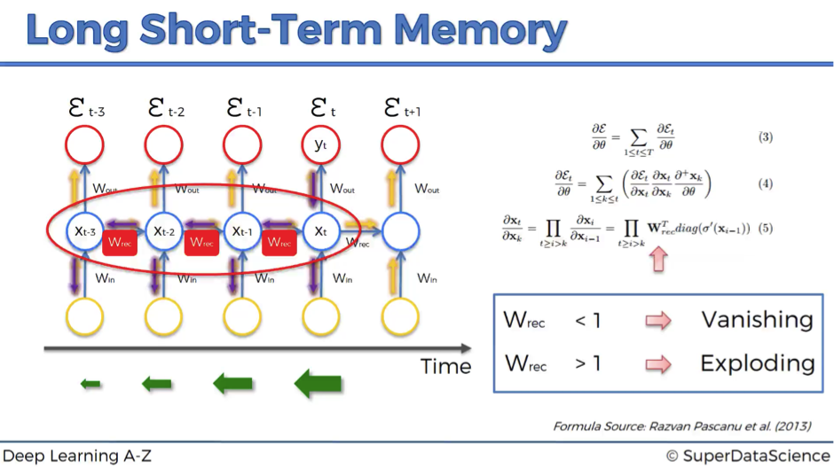
We’ve also defined that as a rule of thumb, if wrec is small – the gradient is vanishing, and if wrec is large – the gradient is exploding.
But what’s “large” and “small” in this context? In fact, we can say that we have a vanishing gradient if wrec < 1 and exploding gradient if wrec > 1.
Then, what’s the first thing that comes to your mind to solve this problem? Probably, the easiest and fastest solution will be to make wrec = 1. That’s exactly what was done in LSTMs. Of course, this is a very simplified explanation, but in general, making recurrent weight equal to one is the main idea behind LSTMs.
Now, let’s dig deeper into the architecture of LSTMs.
LSTM Architecture
Long short-term memory network was first introduced in 1997 by Sepp Hochreiter and his supervisor for a Ph.D. thesis Jurgen Schmidhuber. It suggests a very elegant solution to the vanishing gradient problem.
Overview
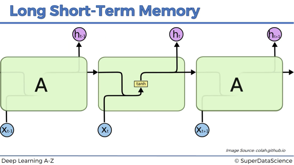
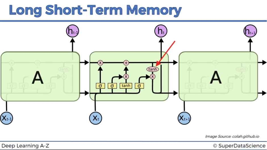
To provide you with the most simple and understandable illustrations of LSTM networks, we are going to use images created by Christopher Olah for his blog post, where he does an amazing job on explaining LSTMs in simple terms.
So, the first image below demonstrates how a standard RNN looks like from the inside.
The hidden layer in the central block receives input xt from the input layer and also from itself in time point t-1, then it generates output ht and also another input for itself but in time point t+1.
This is a standard architecture that doesn’t solve a vanishing gradient problem.
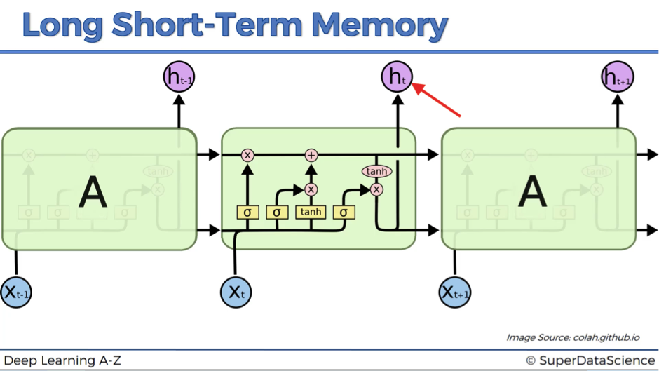
The next image shows how LSTMs look like. This might seem very complex at the beginning, but don’t worry!
We’re going to walk you through this architecture and explain in detail, what’s happening here. By the end of this article, you’ll be completely comfortable with navigating LSTMs.
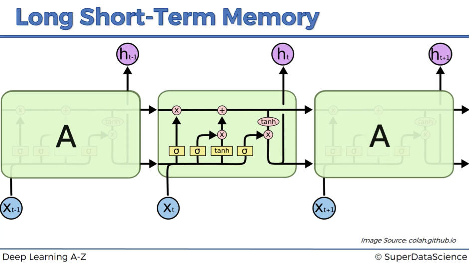
As you might recall, we’ve started with the claim that in LSTMs wrec = 1. This feature is reflected as a straight pipeline on the top of the scheme and is usually referenced as a memory cell. It can very freely flow through time. Though sometimes it might be removed or erased, sometimes some things might be added to it. Otherwise, it flows through time freely, and therefore when you backpropagate through these LSTMs, you don’t have that problem of the vanishing gradient.
Notation
Let’s begin with a few words on the notation:
- ct-1 stands for the input from a memory cell in time point t;
- xt is an input in time point t;
- ht is an output in time point t that goes to both the output layer and the hidden layer in the next time point.
Thus, every block has three inputs (xt, ht-1, and ct-1) and two outputs (ht and ct). An important thing to remember is that all these inputs and outputs are not single values, but vectors with lots of values behind each of them.
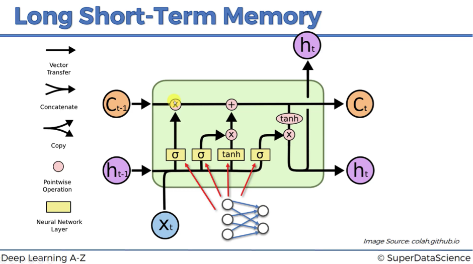
Let’s continue our journey through the legend:
- Vector transfer: any line on the scheme is a vector.
- Concatenate: two lines combining into one, as for example, the vectors from ht-1 and xt. You can imagine this like two pipes running in parallel.
- Copy: the information is copied and goes into two different directions, as for example, at the right bottom of the scheme, where output information is copied in order to arrive at two different layers ht.

- Pointwise operation: there are five pointwise operations on the scheme and they are of three types:
- “x” or valves (forget valve, memory valve, and output valve) – points on the scheme, where you can open your pipeline for the flow, close it or open to some extent. For instance, forget valve at the top right of the above scheme is controlled by the layer operation s. Based on a decision of this sigmoid activation function (ranging from 0 to 1), the valve will be closed, open or closed to some extent. If it’s open, memory flows freely from ct-1 to ct. If it’s closed, then memory is cut off, and probably new memory will be added further in the pipeline, where another pointwise operation is depicted.
- “+” – t-shaped joint, where you have memory going through and you can add additional memory if the memory valve below this joint is open.
- “tanh” – responsible for transforming the value to be within the range from -1 to 1 (required due to certain mathematical considerations).
- Neural Network Layer: layer operations, where you’ve got layer coming in and layer coming out
Walk through the architecture
Now we are ready to look into the LSTM architecture step by step:
- We’ve got new value xt and value from the previous node ht-1 coming in.
- These values are combined together and go through the sigmoid activation function, where it is decided if the forget valve should be open, closed or open to some extent.
- The same values, or actually vectors of values, go in parallel through another layer operation “tanh”, where it is decided what value we’re going to pass to the memory pipeline, and also sigmoid layer operation, where it is decided, if that value is going to be passed to the memory pipeline and to what extent.
- Then, we have a memory flowing through the top pipeline. If we have forget valve open and memory valve closed then the memory will not change. Otherwise, if we have forget valve closed and memory valve open, the memory will be updated completely.
- Finally, we’ve got xt and ht-1 combined to decide what part of the memory pipeline is going to become the output of this module.
That’s basically, what’s happening within the LSTM network. As you can see, it has a pretty straightforward architecture, but let’s move on to a specific example to get an even better understanding of the Long Short-Term Memory networks.
Example Walkthrough
You might remember the translation example from one of our previous articles. Recall that when we change the word “boy” to “girl” in the English sentence, the Czech translation has two additional words changed because in Czech the verb form depends on the subject’s gender.

So, let’s say the word “boy” is stored in the memory cell ct-1. It is just flowing through the module freely if our new information doesn’t tell us that there is a new subject.
If for instance, we have a new subject (e.g., “girl”, “Amanda”), we’ll close the forget valve to destroy the memory that we had. Then, we’ll open a memory valve to put a new memory (e.g., name, subject, gender) to the memory pipeline via the t-joint.
If we put the word “girl” into the memory pipeline, we can extract different elements of information from this single piece: the subject is female, singular, the word is not capitalized, has 4 letters etc.
Next, the output valve facilitates the extraction of the elements required for the purposes of the next word or sentence (gender in our example). This information will be transferred as an input to the next module and it will help the next module to decide on the best translation given the subject’s gender.
That’s how LSTM actually works.
Additional Reading
First of all, you can definitely reference the original paper:
- Long Short-Term Memory by Sepp Hochreiter and Jurgen Schmidhuber (1997).
Alternatively, if you don’t want to get that deep into mathematics, there are two great blog posts with very good explanations of LSTMs:
- Understanding LSTM Networks by Christopher Olah (2015).
- Understanding LSTM and its diagrams by Shi Yan (2016).
That’s it for LSTM architecture. Hopefully, you are now much more comfortable with this advanced deep learning topic. If you are looking for some more practical examples of LSTM’s application, move on to our next article.
LSTM Practical Intuition
Now we are going to dive inside some practical applications of Long Short-Term Memory networks (LSTMs).
How do LSTMs work under the hood? How do they think? And how do they come up with the final output?
That’s going to be quite an interesting and at the same time a bit of magical experience.
In our journey, we will use examples from the Andrej Karpathy’s blog, which demonstrates the results of his amazing research on the effectiveness of recurrent neural networks. You should definitely check it out to feel the magic of deep learning and in particular, LSTMs.
So, let’s get started!
Neuron Activation
Here is our LSTM architecture. To start off, we are going to be looking at the tangent function tanh and how it fires up. As you remember, its value ranges from -1 to 1. In our further images, “-1” is going to be red and “+1” is going to be blue.
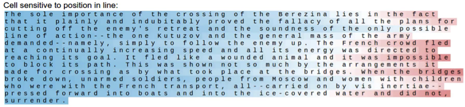
Below is the first example of LSTM “thinking”. The image includes a snippet from “War and Peace” by Leo Tolstoy. The text was given to RNN, and it learned to read it and predict what text is coming next.
As you can see, this neuron is sensitive to position in line. When you get towards the end of the line, it is activating. How does it know that it is the end of the line? You have about 80 symbols per line in this novel. So, it’s counting how many symbols have passed and that’s the way it’s trying to predict when the new line character is coming up.
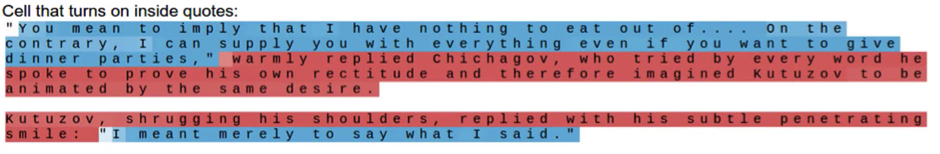
The next cell recognizes direct speech. It’s keeping track of the quotation marks and is activating inside the quotes.
This is very similar to our example where the network was keeping track of the subject to understand if it is male or female, singular or plural, and to suggest the correct verb forms for the translation. Here we observe the same logic. It’s important to know if you are inside or outside the quotes because that affects the rest of the text.
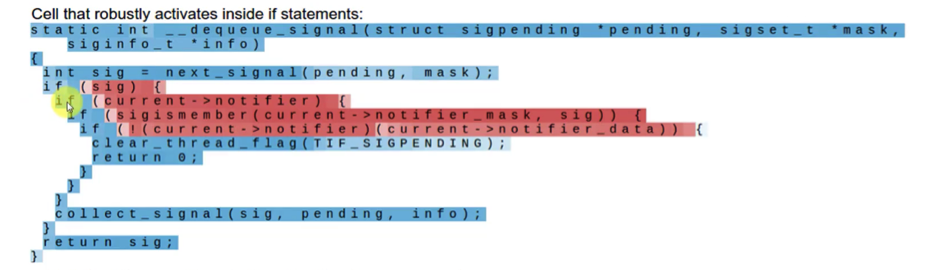
On the next image, we have a snippet from the code of the Linux operating system. This example refers to the cell that activates inside if-statements. It’s completely dormant everywhere else, but as soon as you have an if-statement, it activates. Then, it’s only active for the condition of the if-statement and it stops being active at the actual body of the if-statement. That’s can be important because you’re anticipating the body of the if-statement.
The next cell is sensitive to how deep you are inside of the nested expression. As you go deeper, and the expression gets more and more nested, this cell keeps track of that.
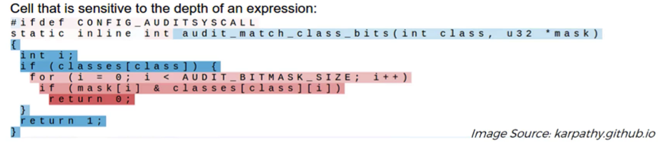
It’s very important to remember that none of these is actually hardcoded into the neural network. All of these is learned by the network itself through thousands and thousands of iterations.
The network kind of thinks: okay, I have this many hidden states, an out of them I need to identify, what’s important in a text to keep track off. Then, it identifies that in this particular text understanding how deep you’re inside a nested statement is important. Therefore, it assigns one of its hidden states, or memory cells, to keep track of that.
So, the network is really evolving on itself and deciding how to allocate its resources to best complete the task. That’s really fascinating!
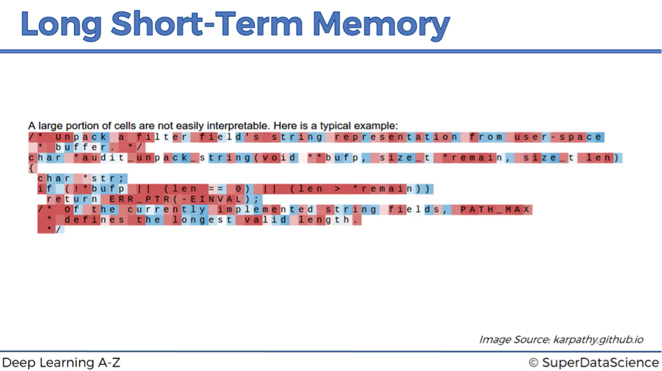
The next image demonstrates an example of the cell that you can’t really understand, what it’s doing. According to Andrej Karpathy, about 95% of the cells are like this. They are doing something, but that’s just not obvious to humans, while it makes sense for machines.
Output
Now let’s move to the actual output ht. This is the resulting value after it passed the tangent function and the output valve.
So, what do we actually see in the next image?
This is a neural network that is reading a page from Wikipedia. This result is a bit more detailed. The first line shows us if the neuron is active (green color) or not (blue color), while the next five lines say us, what the neural network is predicting, particularly, what letter is going to come next. If it’s confident about its prediction, the color of the corresponding cell is red and if it’s not confident – it is light red.
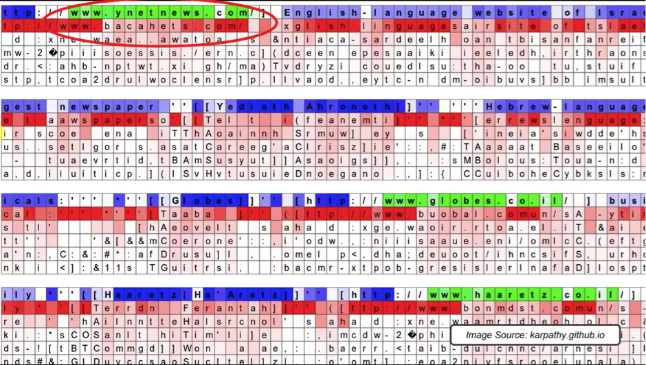
What do you think this specific hidden state in the neural network is looking out for?
Yes, it’s activating inside URLs!
The first row demonstrates the neuron’s activation inside the URL www.ynetnews.com. Then, below each of the letter you can see, what is the network’s prediction for the next letter.
For example, after the first “w” it’s pretty confident that the next letter will be “w” as well. Conversely, its prediction about the letter or symbol after “.” is very unsure because it could actually be any website.
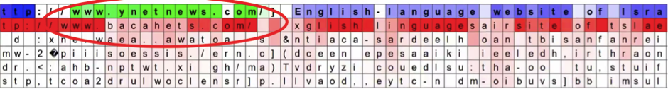
As you see from the image, the network continues generating predictions even when the actual neuron is dormant. See, for example, how it was able to predict the word “language” just from the first two letters.
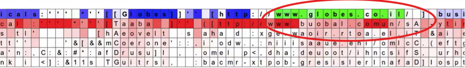
The neuron activates again in the third row, when another URL appears (see the image below). That’s quite an interesting case.
You can observe that the network was pretty sure that the next letter after “co” should be “m” to get “.com”, but it was another dot instead.
Then, the network predicted “u” because the domain “co.uk” (for the United Kingdom) is quite popular. And again, this was the wrong prediction because the actual domain was “co.il” (for Israel), which was not at all considered by the neural network even as 2nd, 3rd, 4th or 5th best guess.
This is how to look at this pictures that Andrej has created. There is a couple more of such examples in his blog.
Hopefully, you are now much more comfortable about what’s going on inside the neural network, when it’s thinking and processing information.
Additional Reading
In terms of references and additional reading, we’ve got Andrej Karpaty’s blog and a research paper prepared by Andrej Karpathy in cooperation with his colleagues:
- The Unreasonable Effectiveness of Recurrent Neural Networks by Andrej Karpathy (2015).
- Visualizing and Understanding Recurrent Networks by Andrey Karpathy et al. (2015).
This is actually a very exciting reading. You can see how the researchers “open up the brain” of the neural networks and monitor what’s happening in one specific neuron.
You actually feel from the language that this is if they are exploring some alien and how it thinks.
But wait! Humans created these LSTMs! However, they’ve become so advanced and complex, that we need now to study them as if they are separate beings.
Isn’t this exciting? Make sure to check the articles if you also want to feel this magic.
LSTM Variation
Have you checked all our articles on Recurrent Neural Networks (RNNs)? Then you should be already pretty much comfortable with the concept of Long Short-Term Memory networks (LSTMs).
Let’s wind up our journey with a very short article on LSTM variations.
You may encounter them sometimes in your work. So, it could be really important for you to be at least aware of these other LSTM architectures.
Here is the standard LSTM that we discussed.
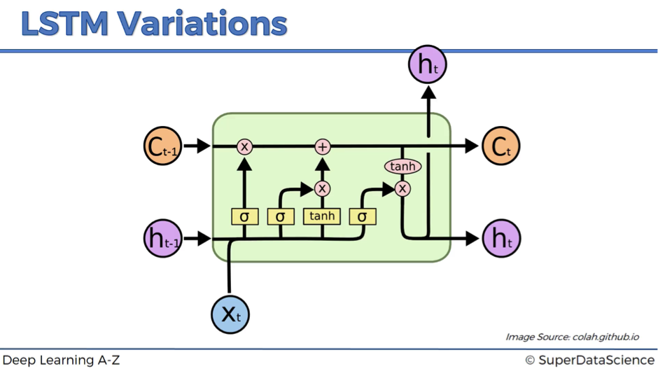
Now let’s have a look at a couple of variations.
Variation #1
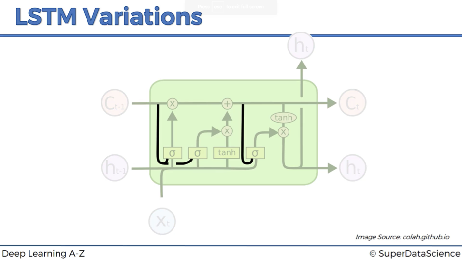
In variation #1, we add peephole connections – the lines that feed additional input about the current state of the memory cell to the sigmoid activation functions.
Variation #2
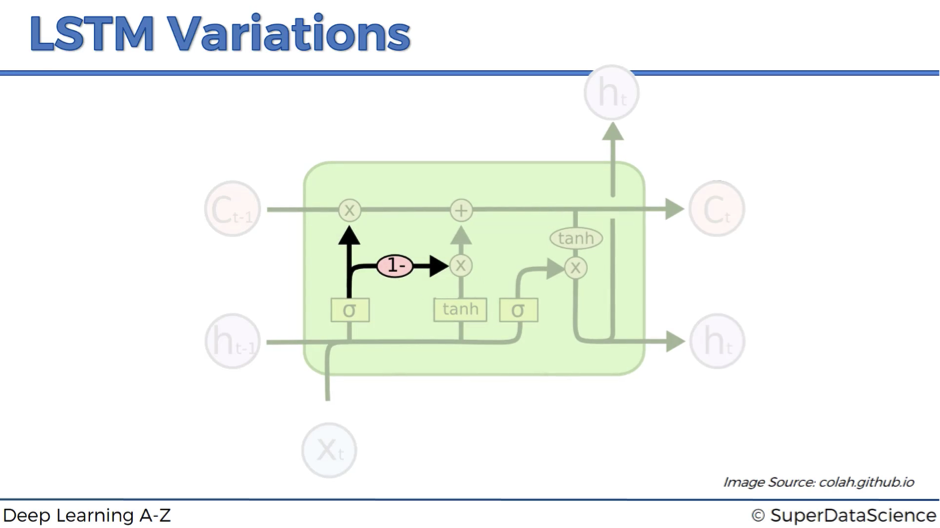
In variation #2, we connect forget valve and memory valve. So, instead of having separate decisions about opening and closing the forget and memory valves, we have a combined decision here.
Basically, whenever you close the memory off (forget valve = 0), you have to put something in (memory valve = 1 – 0 = 1), and vice versa.
Variation #3
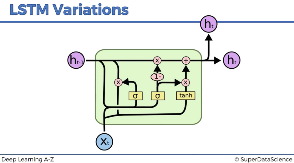
Variation #3 is usually referred to as Gated Recurrent Unit (GRU). This modification completely gets rid of the memory cell and replaces it with the hidden pipeline. So, here instead of having two separate values – one for the memory and one for the hidden state – you have only one value.
It might look quite complex, but in fact, the resulting model is simpler than the standard LSTM. That’s why this modification becomes increasingly popular. We have discussed three LSTM modifications, which are probably the most notable. However, be aware that there are lots and lots of others LSTM variations out there.
Additional Reading
And finally, another good paper to check out:
- LSTM: A Search Space Odyssey by Klaus Greff et al. (2015).
This is a very good comparison of popular LSTM variants. Check it out, if interested!
That’s it! Thanks for following this guide on Recurrent Neural Networks, we hope you’ve enjoyed, learned and challenged yourself on this section of Deep Learning A-Z.
That was step 3 in our journey of Deep Learning. If you liked Recurrent Neural Networks (CNNs) then you’ll be ready for Self Organizing Maps.