
So you want to learn Convolutional Neural Networks? Well you’ve come to the right place…. The Ultimate Guide to Convolutional Neural Networks is here!
If you go past the “convoluted” vocabulary (pun obviously intended), you will find that the plan of attack is set up in a way that will really help you dissect and absorb the concept.
The end goal is for you to understand what these networks are and how they operate.
As we get into that, you will get to see the differences and the similarities between Convolutional Neural Networks and your own brain, most particularly in the context of image recognition.
Convolutional Neural Networks – Plan of Attack
These are the steps (our Plan of Attack) we’ll follow for you to master Convolutional Neural Networks and consequently Deep Learning:
CNNs aren’t an easy feat to master. This is the first step in your journey – so get a grip on the basics before getting started.
A Convolutional Neural Networks Introduction so to speak.
The first building block in our plan of attack is convolution operation. In this step, we will touch on feature detectors, which basically serve as the neural network’s filters. We will also discuss feature maps, learning the parameters of such maps, how patterns are detected, the layers of detection, and how the findings are mapped out.
The second part of this step will involve the Rectified Linear Unit or ReLU. We will cover ReLU layers and explore how linearity functions in the context of Convolutional Neural Networks.
Not necessary for understanding CNN’s, but there’s no harm in a quick lesson to improve your skills.
In this part, we’ll cover pooling and will get to understand exactly how it generally works. Our nexus here, however, will be a specific type of pooling; max pooling. We’ll cover various approaches, though, including mean (or sum) pooling. This part will end with a demonstration made using a visual interactive tool that will definitely sort the whole concept out for you.
This will be a brief breakdown of the flattening process and how we move from pooled to flattened layers when working with Convolutional Neural Networks.
In this part, everything that we covered throughout the section will be merged together. By learning this, you’ll get to envision a fuller picture of how Convolutional Neural Networks operate and how the “neurons” that are finally produced learn the classification of images.
In the end, we’ll wrap everything up and give a quick recap of the concept covered in the section. If you feel like it will do you any benefit (and it probably will), you should check out the extra tutorial in which Softmax and Cross-Entropy are covered. It’s not mandatory for the course, but you will likely come across these concepts when working with Convolutional Neural Networks and it will do you a lot of good to be familiar with them.
A little extra to enhance your understanding of Convolutional Neural Networks. Ready? Let’s get started!
What Are Convolutional Neural Networks?
In this tutorial, we’re going to answer the following questions in the most basic sense before expanding on each of them in the coming tutorials in this section:
- How do our brains work?
- How do convolutional neural networks work?
- How do they scan images?
- How do neural networks read facial expressions?
- What are the steps that constitute the convolutional neural network’s process?
Let’s begin.
First question: How does the human brain work?
More precisely, how do we recognize the objects and the people around us or in images? Understanding this is a large part of understanding convolutional neural networks. In a nutshell, our brains depend on detecting features and they categorize the objects we see accordingly.
You have probably been through hundreds of situations in your life where you looked at something instantaneously, made it out to be something, and then after looking at it more thoroughly, you realize that it is actually something completely different.
What happens there is that your brain detects the object for the first time, but because the look was brief, your brain does not get to process enough of the object’s features so as to categorize it correctly.
Let’s start with a brief game of optical illusions.
Look at the following images:
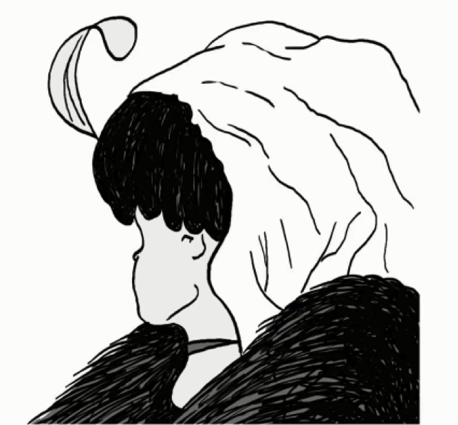
Do you see an old lady looking down or a young lady staring away?
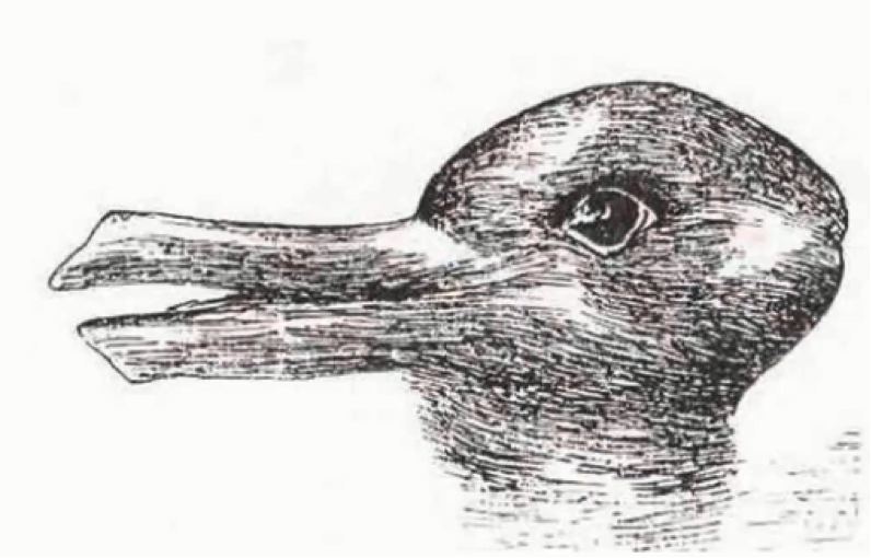
Do you see a rabbit or a duck?
That’s enough with the games. The point to be made here is that your brain classifies objects in an image based on the features that it detects first.
The previous images were designed so that what you see in them depends on the line and the angle that your brain decides to begin its “feature detection” expedition from.
As we proceed in our section on convolutional neural networks, you will realize the staggering degree of similarity between how these networks operate and how your brain does. They, too, categorize objects or images based on the set of features that are passed through them and that they manage to detect.
Now let’s look at an example of a test set that is fed to a convolutional neural networks and the results that the network gave.

It’s worth noting that the four categories that show up on this guess list are far from being the only categories that the network gets to choose from.
It usually has to sift through hundreds, or more likely thousands, of categories until it shortlists the ones you see in the image above, which it then ranks according to their probability of being the right category for the presented image.
You can see that the network was not as certain about the last image as it was about the first two. We can infer from this that one major thing about convolutional neural networks that you should always take into account is that the poor bastards often get confused at least in their earlier stages of training.
Just like your brain oftentimes mistakenly categorizes objects at first sight, convolutional neural networks are prone to the same indecision when presented with an object or an image from an angle that can easily place it under more than one category.
As a matter of fact, with that very image in the screenshot above, many humans are uncertain of what the object actually is. As we can see, the correct answer was “hand glass,” not a pair of scissors as the network categorized it.
Why Convolutional Neural Networks Are So Important
To understand this, you can ask yourself a couple of simple questions:
- How do self-driving cars recognize other cars as well as pedestrians and street objects?
- How did Facebook go from making you tag people in images yourself, to being able to identify your friends and automatically tag them as it does now?
And the answer to both questions would be: through the magic of convolutional neural networks.
So, how do convolutional neural networks actually operate?
The first thing you need to know here is the elements that are included in the operation:
- Input image
- Convolutional Neural Network
- Output label (image class)
These elements interact in the following manner:
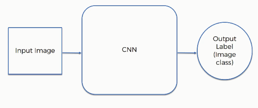
We already saw how convolutional neural networks can categorize images according to the objects included in them. That is not their only use, however.
For example, convolutional neural networks can be used in detected human emotions in an image. You provide them with someone’s photo, and they produce a classification to the effect of what that person seems to be feeling.
Of course, this requires a somewhat more advanced level of training since being able to infer someone’s emotions from their facial expressions is often quite a puzzling task to humans themselves.
Naturally, only a small portion of people can do so with a fairly high degree of success.
How Convolutional Neural Networks Scan Images
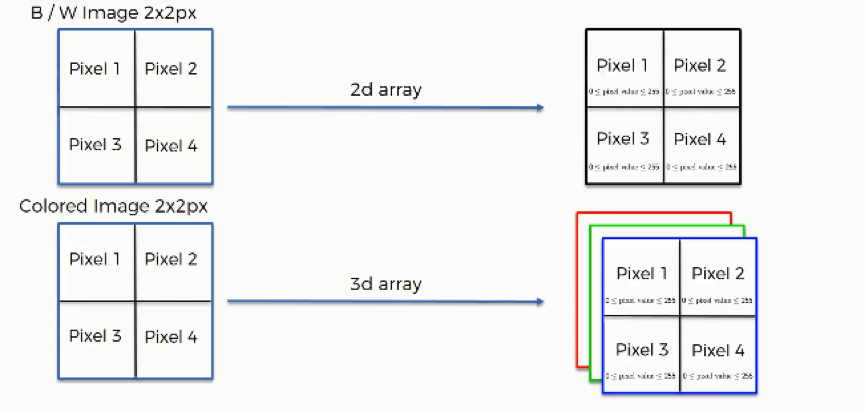
Before getting into the details of this operation, you should first keep in mind that the way black & white images are scanned differs in one major way from how colored images are. We’re going to examine each of them separately, but first, let’s look at the similarities.
Both types of images are similar in the following respects:
- Each pixel contains 8 bits (1 byte) of information.
- Colors are represented on a scale from 0 to 255. The reason for this is that bits are binary units, and since we have 8 of these per byte, a byte can have any of 256 (2^8) possible values. Since we count 0 as the first possible value, we can go up to 255.
- In this model, 0 is pitch black and 255 is pure white, and in between are the various (definitely more than 50!) shades of gray.
- The network does not actually learn colors. Since computers understand nothing but 1’s and 0’s, the colors’ numerical values are represented to the network in binary terms.
Now let’s delve into the major difference that we mentioned above.
Black & white images are two-dimensional, whereas colored images are three-dimensional. The difference this makes is in the value assigned to each pixel when presented to the neural network. In the case of two-dimensional black & white images, each pixel is assigned one number between 0 and 255 to represent its shade.
On the other hand, each pixel inside a colored image is represented on three levels. Since any color is a combination of red, green, and blue at different levels of concentration, a single pixel in a colored image is assigned a separate value for each of these layers.
That means that the red layer is represented with a number between 0 and 255, and so are the blue and the green layers. They are then presented in an RGB format. For example, a “hot pink” pixel would be presented to the neural network as (255, 105, 180).
Detecting Facial Expressions
Let’s look at a case in which a convolutional neural network is asked to read a human smile. For the purpose of simplification, the following figure shows an extremely basic depiction of a human (loosely speaking, of course) smile.
Matters obviously get more complex when we’re trying to feed the network pictures of actual human beings.
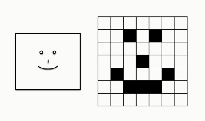

As you can see, the grid table on the far right shows all of the pixels valued at 0’s while only the parts where the smiley face appears are valued at 1. This differs from the 8-bit model we just discussed, again, for the sake of breaking down the concept.
In the table above, white cells are represented as 0’s, and black cells are represented as 1’s, which means that there are no other possible shades that can appear in this image.
What we do when training a convolutional neural network to detect smiles is to teach it the patterns of 0’s and 1’s that are normally associated with the shape of a smile.
If you look at the arc of 1’s that ends in the second row from the bottom you would be able to recognize the smile.
The steps that go into this process are broken down as follows:
You will probably find these terms to be too much to digest at the moment, which is quite normal at this point. As we go through the next tutorials, you will get to understand what each of them actually means.
Additional Reading
In the meantime, if you want to geek out on some extra material, you should check out this paper titled “Gradient-Based Learning Applied to Document Recognition” by Yann LeCun and others.
LeCun is considered to be one of the founding fathers of the field of convolutional neural networks, and he was the first person to head the Facebook AI Research organization in New York before stepping down earlier this year.
So, if there is someone who can give you the gist of the subject, it is definitely this guy.
Now it’s time for you to do some reading on the topic so you can get more familiar with the broad concept of convolutional neural networks, and in the next tutorial we will begin to break it down into its four basic steps.
Step 1 – Convolution Operation
In this tutorial, we are going to learn about convolution, which is the first step in the process that convolutional neural networks undergo. We’ll learn what convolution is, how it works, what elements are used in it, and what its different uses are.
Get ready!
What is convolution?
In purely mathematical terms, convolution is a function derived from two given functions by integration which expresses how the shape of one is modified by the other. That can sound baffling as it is, but to make matters worse, we can take a look at the convolution formula:

If you don’t consider yourself to be quite the math buff, there is no need to worry since this course is based on a more intuitive approach to the concept of convolutional neural networks, not a mathematical or a purely technical one.
Those of you who have practiced any field that entails signal processing are probably familiar with the convolution function.
If you want to do some extra work on your own to scratch beneath the surface with regard to the mathematical aspects of convolution, you can check out this 2017 University professor Jianxin Wu titled “Introduction to Convolutional Neural Networks.”
Let’s get into the actual convolution operation in the context of neural networks. The following example will provide you with a breakdown of everything you need to know about this process.
The Convolution Operation
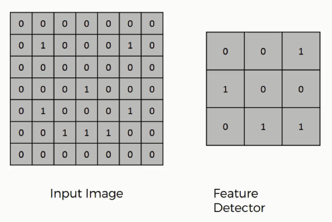
Here are the three elements that enter into the convolution operation:
- Input image
- Feature detector
- Feature map
As you can see, the input image is the same smiley face image that we had in the previous tutorial. Again, if you look into the pattern of the 1’s and 0’s, you will be able to make out the smiley face in there.
Sometimes a 5×5 or a 7×7 matrix is used as a feature detector, but the more conventional one, and that is the one that we will be working with, is a 3×3 matrix. The feature detector is often referred to as a “kernel” or a “filter,” which you might come across as you dig into other material on the topic.
It is better to remember both terms to spare yourself the confusion. They all refer to the same thing and are used interchangeably, including in this course.
How exactly does the convolution operation work?
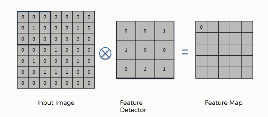
You can think of the feature detector as a window consisting of 9 (3×3) cells. Here is what you do with it:
- You place it over the input image beginning from the top-left corner within the borders you see demarcated above, and then you count the number of cells in which the feature detector matches the input image.
- The number of matching cells is then inserted in the top-left cell of the feature map.
- You then move the feature detector one cell to the right and do the same thing. This movement is called a and since we are moving the feature detector one cell at time, that would be called a stride of one pixel.
- What you will find in this example is that the feature detector’s middle-left cell with the number 1 inside it matches the cell that it is standing over inside the input image. That’s the only matching cell, and so you write “1” in the next cell in the feature map, and so on and so forth.
- After you have gone through the whole first row, you can then move it over to the next row and go through the same process.
It’s important not to confuse the feature map with the other two elements. The cells of the feature map can contain any digit, not only 1’s and 0’s. After going over every pixel in the input image in the example above, we would end up with these results:
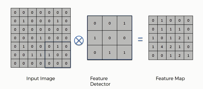
By the way, just like feature detector can also be referred to as a kernel or a filter, a feature map is also known as an activation map and both terms are also interchangeable.
What is the point from the convolution operation?
There are several uses that we gain from deriving a feature map. These are the most important of them: Reducing the size of the input image, and you should know that the larger your strides (the movements across pixels), the smaller your feature map.
In this example, we used one-pixel strides which gave us a fairly large feature map.
When dealing with proper images, you will find it necessary to widen your strides. Here we were dealing with a 7×7 input image after all, but real images tend to be substantially larger and more complex.
That way you will make them easier to read.
Do we lose information when using a feature detector?
The answer is YES. The feature map that we end up with has fewer cells and therefore less information than the original input image. However, the very purpose of the feature detector is to sift through the information in the input image and filter the parts that are integral to it and exclude the rest.
Basically, it is meant to separate the wheat from the chaff.
Why do we aim to reduce the input image to its essential features?
Think of it this way. What you do is detect certain features, say, their eyes and their nose, for instance, and you immediately know who you are looking at.
These are the most revealing features, and that is all your brain needs to see in order to make its conclusion. Even these features are seen broadly and not down to their minutiae.
If your brain actually had to process every bit of data that enters through your senses at any given moment, you would first be unable to take any actions, and soon you would have a mental breakdown. Broad categorization happens to be more practical.
Convolutional neural networks operate in exactly the same way.
How do convolutional neural networks actually perform this operation?
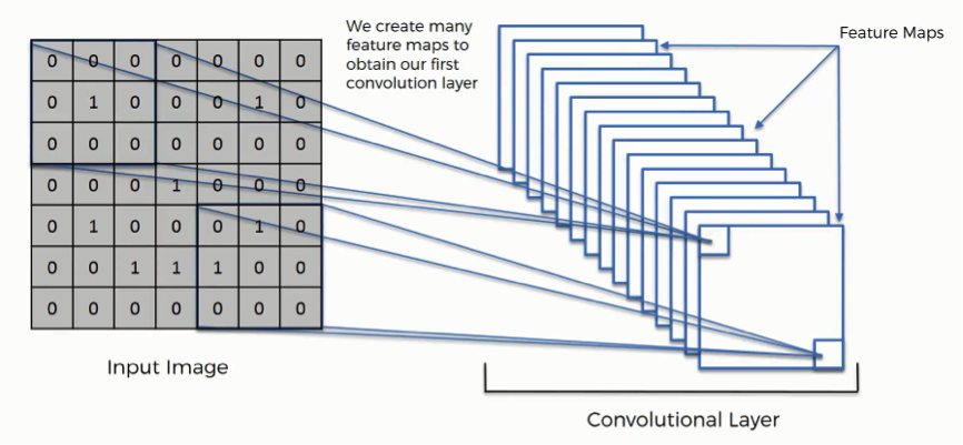
The example we gave above is a very simplified one, though. In reality, convolutional neural networks develop multiple feature detectors and use them to develop several feature maps which are referred to as convolutional layers (see the figure below).
Through training, the network determines what features it finds important in order for it to be able to scan images and categorize them more accurately.
Based on that, it develops its feature detectors. In many cases, the features considered by the network will be unnoticeable to the human eye, which is exactly why convolutional neural networks are so amazingly useful. With enough training, they can go light years ahead of us in terms of image processing.
What are other uses of convolution matrices?
There’s another use for convolution matrix, which is actually part of the reason why they are called “filters.” The word here is used in the same sense we use it when talking about Instagram filters.
You can actually use a convolution matrix to adjust an image. Here are a few examples of filters being applied to images using these matrices.
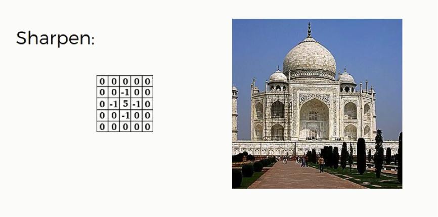
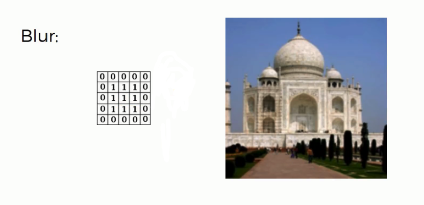
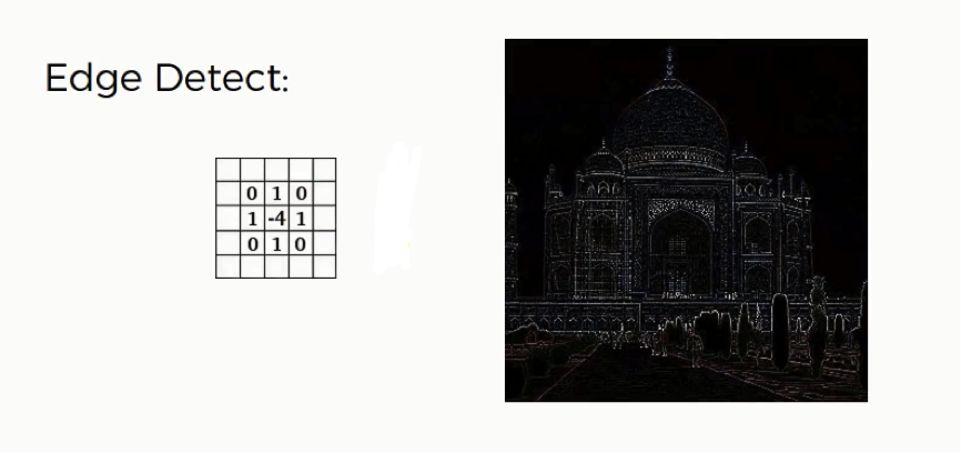
There is really little technical analysis to be made of these filters and it would be of no importance to our tutorial. These are just intuitively formulated matrices. The point is to see how applying them to an image can alter its features in the same manner that they are used to detect these features.
What’s next?
That’s all you need to know for now about the convolution operation. In our next tutorial, we will go through the next part of the convolution step; the ReLU layer.
Step 1(b): The Rectified Linear Unit (ReLU)
The Rectified Linear Unit, or ReLU, is not a separate component of the convolutional neural networks’ process.
It’s a supplementary step to the convolution operation that we covered in the previous tutorial. There are some instructors and authors who discuss both steps separately, but in our case, we’re going to consider both of them to be components of the first step in our process.
If you’re done with the previous section on artificial neural networks, then you should be familiar with the rectifier function that you see in the image below.
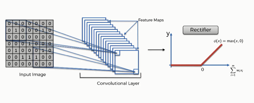
The purpose of applying the rectifier function is to increase the non-linearity in our images.
The reason we want to do that is that images are naturally non-linear.
When you look at any image, you’ll find it contains a lot of non-linear features (e.g. the transition between pixels, the borders, the colors, etc.).
The rectifier serves to break up the linearity even further in order to make up for the linearity that we might impose an image when we put it through the convolution operation.
To see how that actually plays out, we can look at the following picture and see the changes that happen to it as it undergoes the convolution operation followed by rectification.
The Input Image
This black and white image is the original input image.
Feature Detector
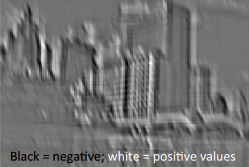
By putting the image through the convolution process, or in other words, by applying to it a feature detector, the result is what you see in the following image.

As you see, the entire image is now composed of pixels that vary from white to black with many shades of gray in between.
Rectification
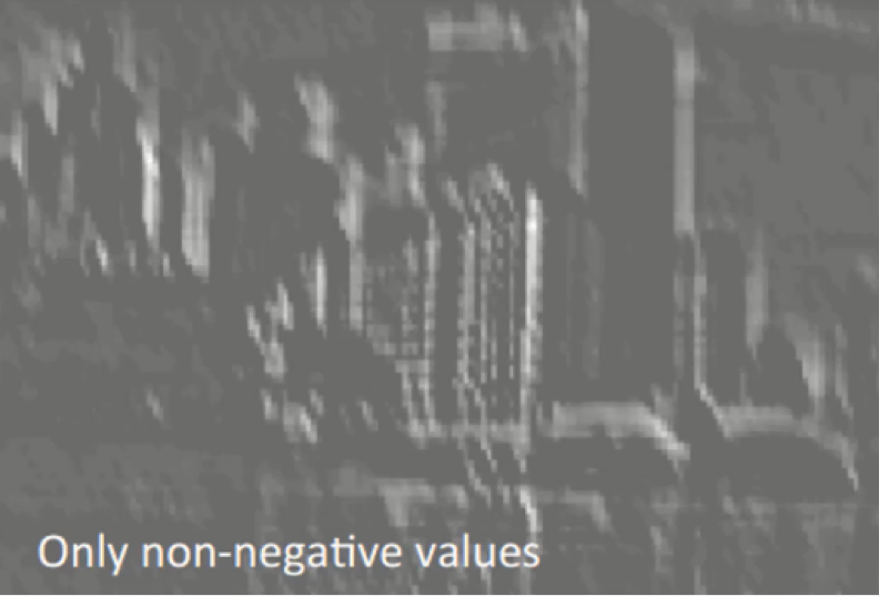
What the rectifier function does to an image like this is remove all the black elements from it, keeping only those carrying a positive value (the grey and white colors).
The essential difference between the non-rectified version of the image and the rectified one is the progression of colors. If you look closely at the first one, you will find parts where a white streak is followed by a grey one and then a black one. After we rectify the image, you will find the colors changing more abruptly.
The gradual change is no longer there. That indicates that the linearity has been disposed of.
You have to bear in mind that the way by which we just examined this example only provides a basic non-technical understanding of the concept of rectification.
The mathematical concepts behind the process are unnecessary here and would be pretty complex at this point.
Additional Readings
If you want to look at the concept through a more mathematical lens, you can check out this 2016 paper by C. C. Jay Kuo titled Understanding Convolutional Neural Networks with a Mathematical Model.
If you’re looking to dig even deeper than that, you can move on to this 2015 paper written by Kaiming He and others from Microsoft Research.
The paper is titled Delving Deep into Rectifiers: Surpassing Human-Level Performance on ImageNet Classification. In this paper, the authors propose a modified form of the rectifier function called the Parametric Rectified Linear Unit (PReLU). It’s quite an interesting read if you’re into the topic.
Step 2 – Max Pooling
What is Max Pooling?
Instead of verbally defining pooling, we’ll start off this tutorial with an example right away.
The Cheetah Example
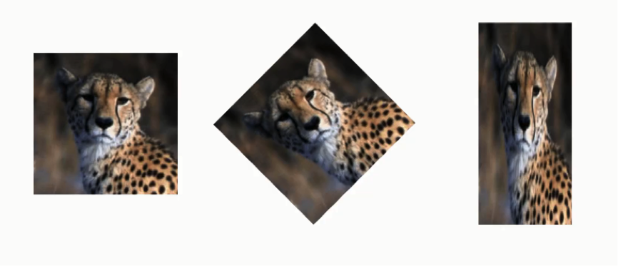
In the example above, the same cheetah image is presented in different ways. It is normal in its first version, rotated in the second, and horizontally squashed in the third. The purpose of max pooling is enabling the convolutional neural network to detect the cheetah when presented with the image in any manner.
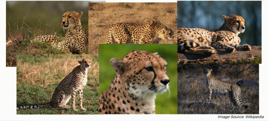
This second example is more advanced. Here we have 6 different images of 6 different cheetahs (or 5, there is 1 that seems to appear in 2 photos) and they are each posing differently in different settings and from different angles.
Again, max pooling is concerned with teaching your convolutional neural network to recognize that despite all of these differences that we mentioned, they are all images of cheetah. In order to do that, the network needs to acquire a property that is known as “spatial variance.”
This property makes the network capable of detecting the object in the image without being confused by the differences in the image’s textures, the distances from where they are shot, their angles, or otherwise.
In order to reach the pooling step, we need to have finished the convolution step, which means that we would have a feature map ready.
Types of Pooling
Before getting into the details, you should know that there are several types of pooling. These include among others the following:
- Mean pooling
- Max pooling
- Sum pooling
Our main focus here will be max pooling.
Pooled Feature Map
The process of filling in a pooled feature map differs from the one we used to come up with the regular feature map. This time you’ll place a 2×2 box at the top-left corner, and move along the row.
For every 4 cells your box stands on, you’ll find the maximum numerical value and insert it into the pooled feature map. In the figure below, for instance, the box currently contains a group of cells where the maximum value is 4.
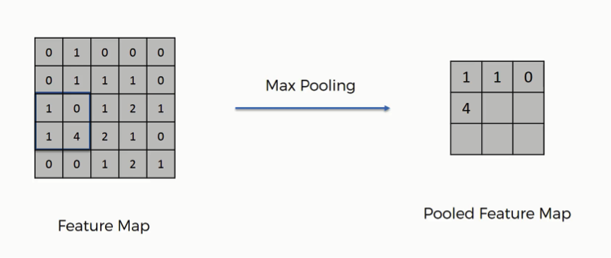
If you remember the convolution operation example from the previous tutorial, we were using strides of one pixel. In this example, we are using 2-pixel strides. That’s why we end up with a 3×3 pooled featured map. Generally, strides of two are most commonly used.
Note that in the third movement along the same row, you will find yourself stuck with one lonely column.
You would still proceed despite the fact that half of your box will be empty. You still find your maximum value and put it in the pooled feature map. In the least step, you will face a situation where the box will contain a single cell. You will take that value to be the maximum value.
Just like in the convolution step, the creation of the pooled feature map also makes us dispose of unnecessary information or features. In this case, we have lost roughly 75% of the original information found in the feature map since for each 4 pixels in the feature map we ended up with only the maximum value and got rid of the other 3. These are the details that are unnecessary and without which the network can do its job more efficiently.
The reason we extract the maximum value, which is actually the point from the whole pooling step, is to account for distortions. Let’s say we have three cheetah images, and in each image the cheetah’s tear lines are taking a different angle.
The feature after it has been pooled will be detected by the network despite these differences in its appearance between the three images. Consider the tear line feature to be represented by the 4 in the feature map above.
Imagine that instead of the four appearing in cell 4×2, it appeared in 3×1. When pooling the feature, we would still end up with 4 as the maximum value from that group, and thus we would get the same result in the pooled version.
This process is what provides the convolutional neural network with the “spatial variance” capability. In addition to that, pooling serves to minimize the size of the images as well as the number of parameters which, in turn, prevents an issue of “overfitting” from coming up.
Overfitting in a nutshell is when you create an excessively complex model in order to account for the idiosyncracies we just mentioned.
Again, this is an abstract explanation of the pooling concept without digging into the mathematical and technical aspects of it.
We can draw an analogy here from the human brain. Our brains, too, conduct a pooling step, since the input image is received through your eyes, but then it is distilled multiple times until, as much as possible, only the most relevant information is preserved for you to be able to recognize what you are looking at.
Additional Reading
If you want to do your own reading on the subject, check out this 2010 paper titled “Evaluation of Pooling Operations in Convolutional Architectures for Object Recognition” by Dominik Scherer and others from the University of Bonn.
It’s a pretty simple read, only 10 pages long, and will boil down the concept of pooling for you just perfectly. You can even skip the second part titled “Related Work” if you find it irrelevant to what you want to understand.
Now, let’s explore a more fun example.
The Number Game
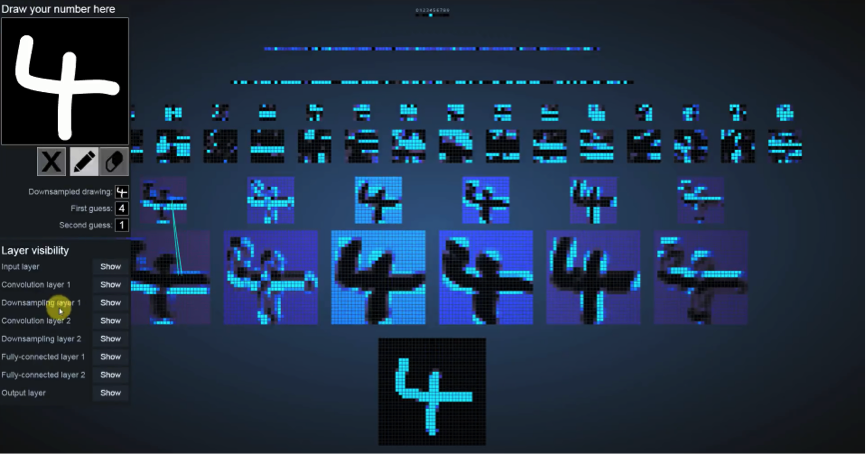
The image above is of an online tool that was developed by You’ll find it hard to find this page using Google, so you can visit it through this link.
Let’s get to it.
What we did in this screenshot is insert a random number, in this case we entered the number 4.
As you see the line-up of images in the middle, the box standing alone in the bottom row represents the input image, and then the row after that represents the convolution operation, followed by the pooling phase.
You’ll see the term “downsampling” used in the “layer visibility” section on the left. Downsampling is simply another word for pooling.
If you look at the various versions of the original image that appear in the convolution row, you’ll be able to recognize the filters being used for the convolution operation and the features that the application is focusing on.
You’ll notice that in the pooling row, the images have more or less the same features as their convolved versions minus some information. You can still recognize it as the same image.
On a side note:
- You can ignore the other rows for now since we haven’t covered these processes yet. Just keep in mind that, like pooling was similar in its steps to the convolution operation, these, too, are just further layers of the same process.
- If you hover with your mouse over any image, it will send out a ray that points at the source of these particular pixels that you’re standing on in the version that came before it (the pooling version will point to the convolution version, and that one would point to the input image.)
You can visit the link above and play around with the tool for a little while until the next tutorial.
Step 3: Flattening
This step is pretty simple, hence the shockingly short tutorial.
After finishing the previous two steps, we’re supposed to have a pooled feature map by now. As the name of this step implies, we are literally going to flatten our pooled feature map into a column like in the image below.
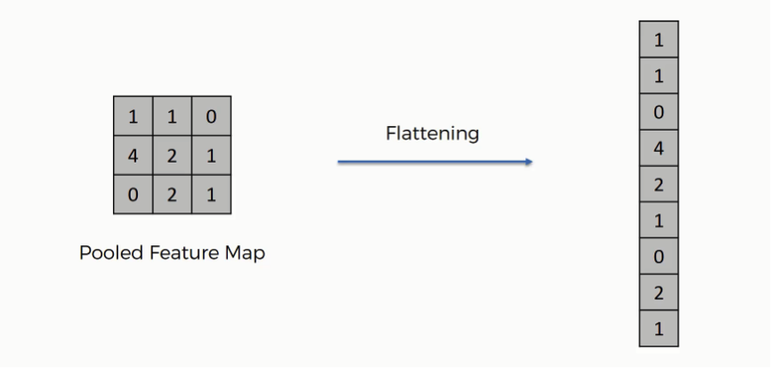
The reason we do this is that we’re going to need to insert this data into an artificial neural network later on.
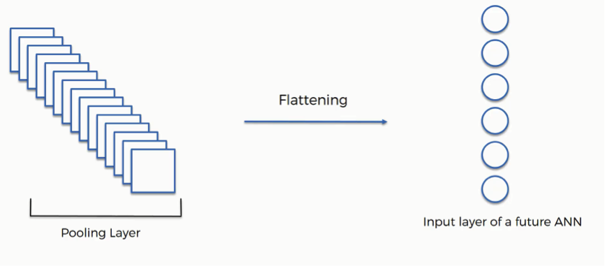
As you see in the image above, we have multiple pooled feature maps from the previous step.
What happens after the flattening step is that you end up with a long vector of input data that you then pass through the artificial neural network to have it processed further.
To sum up, here is what we have after we’re done with each of the steps that we have covered up until now:
- Input image (starting point)
- Convolutional layer (convolution operation)
- Pooling layer (pooling)
- Input layer for the artificial neural network (flattening)
In the next tutorial, we will discuss how this data will be used.
Step 4: Full Connection
Here’s where artificial neural networks and convolutional neural networks collide as we add the former to our latter.
It’s here that the process of creating a convolutional neural network begins to take a more complex and sophisticated turn.
As you see from the image below, we have three layers in the full connection step:
- Input layer
- Fully-connected layer
- Output layer
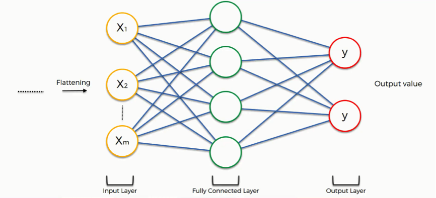
Notice that when we discussed artificial neural networks, we called the layer in the middle a “hidden layer” whereas in the convolutional context we are using the term “fully-connected layer.”
The Full Connection Process
As we said in the previous tutorial, the input layer contains the vector of data that was created in the flattening step. The features that we distilled throughout the previous steps are encoded in this vector.
At this point, they are already sufficient for a fair degree of accuracy in recognizing classes. We now want to take it to the next level in terms of complexity and precision.
What is the aim of this step?
The role of the artificial neural network is to take this data and combine the features into a wider variety of attributes that make the convolutional network more capable of classifying images, which is the whole purpose from creating a convolutional neural network.
We can now look at a more complex example than the one at the beginning of the tutorial.
We’ll explore how the information is processed from the moment it is inserted into the artificial neural network and until it develops its classes (dog, cat).
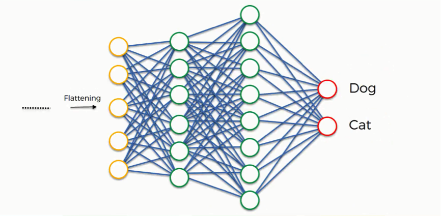
At the very beginning, as you know by now, we have an input image which we convolve, pool, flatten, and then pass through the artificial neural network.
By the end of this channel, the neural network issues its predictions.
Say, for instance, the network predicts the figure in the image to be a dog by a probability of 80%, yet the image actually turns out to be of a cat. An error has to be calculated in this case. In the context of artificial neural networks, we call this calculation a “cost function” or a mean squared error, but as we deal with convolutional neural networks, it is more commonly referred to as a “loss function.”
We use the cross-entropy function in order to achieve that. The cross-entropy function and mean squared errors will be discussed in detail in a separate tutorial, so, if you’re interested in the topic, you can stick around for the extra tutorials at the end of this section. For now, all you need to know is that the loss function informs us of how accurate our network is, which we then use in optimizing our network in order to increase its effectiveness.
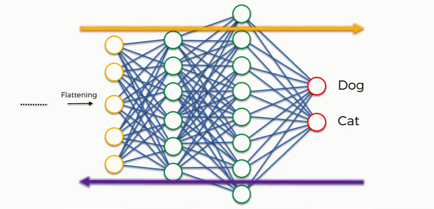
That requires certain things to be altered in our network. These include the weights (the blue lines connecting the neurons, which are basically the synapses), and the feature detector since the network often turns out to be looking for the wrong features and has to be reviewed multiple times for the sake of optimization.
Just as we said when discussing artificial neural networks, the information is then conveyed in the opposite direction as you see in the figure below. As we work to optimize the network, the information keeps flowing back and forth over and over until the network reaches the desired state.
As you’re always reminded, this process is explained here in an intuitive manner, but the science and the mathematics behind it are more complex, of course.
Class Recognition
Up until now, we’ve been discussing examples where the output consists of a single neuron.
Since this one contains two, there are some differences that show up.
Let’s first look at the “dog” class.
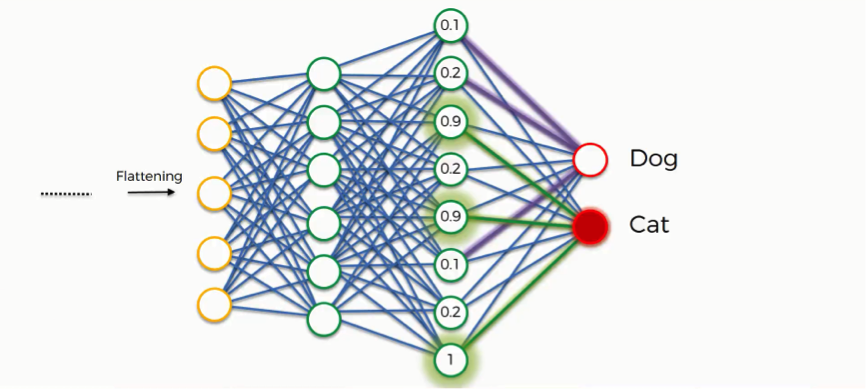
In order to understand how it will play out, we need to check out the weights placed on each synapse linking to this class so that we can tell which attributes/features are most relevant to it.
This full connection process practically works as follows:
- The neuron in the fully-connected layer detects a certain feature; say, a nose.
- It preserves its value.
- It communicates this value to both the “dog” and the “cat” classes.
- Both classes check out the feature and decide whether it’s relevant to them.
In our example, the weight placed on the nose-dog synapse is high (1.0), which means that the network is confident that this is a dog’s nose.
Since the information is constantly flowing in both directions, the “cat” class takes note of this and understands that since this is a dog’s nose, then it simply can’t be a cat’s nose. Even if at first it would have considered the signal saying “small rounded nose” because this might be a cat’s as well as a dog’s nose, now it dismisses this feature.
This happens gradually as it receives the same reading multiple times. The dog class on its part will start focusing more on the attributes carrying the highest weight (the three thick purple lines), and it will ignore the rest.
The same process simultaneously occurs with the cat, enabling it to pick out its own priority features. What we end up with is what you see in the image below. As this process goes on repeat for thousands of times, you find yourself with an optimized neural network.
The Application
The next step becomes putting our network’s efficacy to the test. Say, we give it an image of a dog.
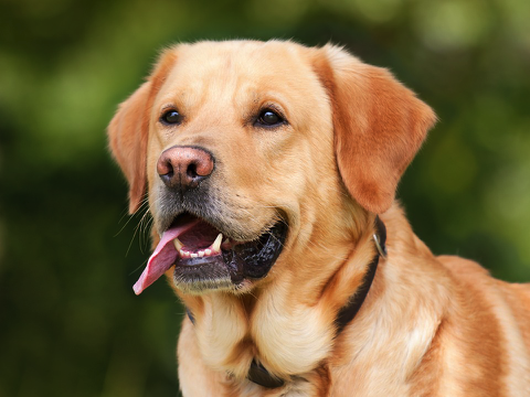
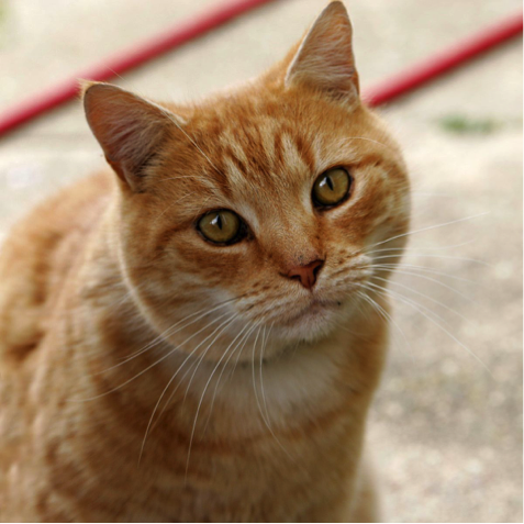
The dog and cat classes at the end of the artificial neural network have absolutely no clue of the image. All they have is what is given to them by the previous layer through the synapses.
By now, each of these classes has three attributes that it’s focusing its attention on.
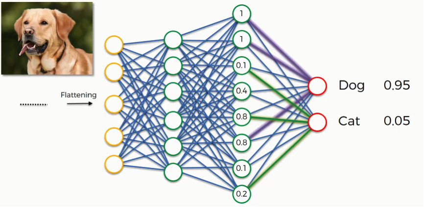
That previous layer passes on which of these features it detects, and based on that information, both classes calculate their probabilities, and that is how the predictions are produced.
As you see in the step below, the dog image was predicted to fall into the dog class by a probability of 0.95 and other 0.05 was placed on the cat class.
Think of it this way: This process is a vote among the neurons on which of the classes the image will be attributed to. The class that gets the majority of the votes wins. Of course, these votes are as good as their weights.
The End of the Convolution Process
Remember this image?
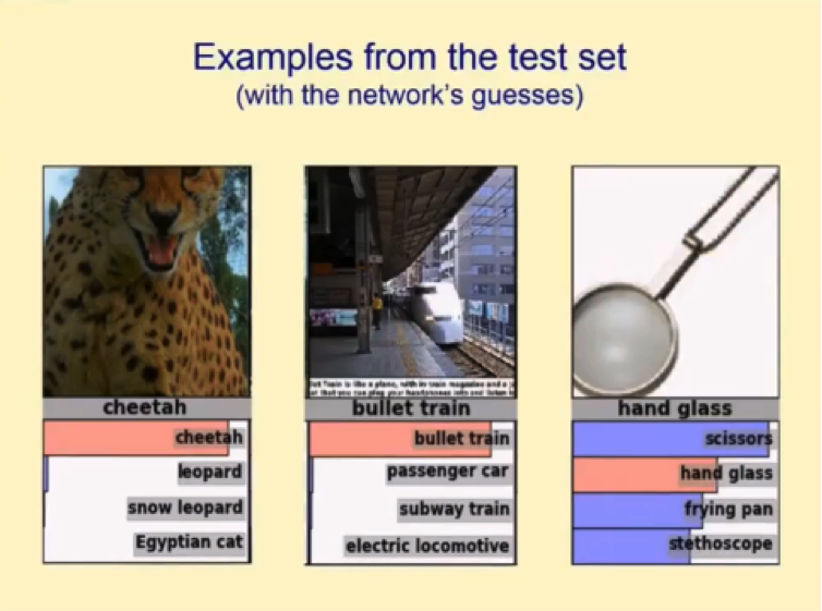
We saw this example in the first tutorial in this section, and by now you have an understanding of the whole process by which these guesses were produced.
Summary
The Convolution Process: A Quick Recap
Since we’re now done with this section, let’s make a quick recap of what we learned about convolutional neural networks. In the diagram below, you can see the entire process of creating and optimizing a convolutional neural network that we covered throughout the section.
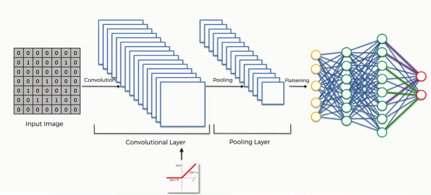
As you see and should probably remember from the previous tutorials, the process goes as follows:
- We start off with an input image.
- We apply filters or feature maps to the image, which gives us a convolutional layer.
- We then break up the linearity of that image using the rectifier function.
- The image becomes ready for the pooling step, the purpose of which is providing our convolutional neural network with the faculty of “spatial invariance” which you’ll see explained in more detail in the pooling tutorial.
- After we’re done with pooling, we end up with a pooled feature map.
- We then flatten our pooled feature map before inserting into an artificial neural network.
Throughout this entire process, the network’s building blocks, like the weights and the feature maps, are trained and repeatedly altered in order for the network to reach the optimal performance that will make it able to classify images and objects as accurately as possible.
By this point, you have acquired all the knowledge you need for you to proceed to the more practical applications of the concept of convolutional neural networks.
Additional Reading
If you’re still craving more on the subject, though, you can always do some extra reading of your own.
This blog post by Adit Deshpande from 2016 titled The 9 Deep Learning Papers You Need To Know About (Understanding CNN’s Part 3) will brief you up on 9 real-life applications of what you learned in this section, and you can then go on to study these examples in more depth.
Granted, you’ll stumble on quite a few concepts that will be brand new for you, but with the knowledge you have now, you’ll be able to manage a general overview on these papers.
Also, as you train more, you can always revisit these case studies every once in a while with your newly-acquired experience.
Softmax & Cross-Entropy
Disclaimer: You should know that this softmax and cross-entropy tutorial is not completely necessary nor is it mandatory for you to proceed in this deep learning course.
That being said, learning about the softmax and cross-entropy functions can give you a tighter grasp of this section’s topic.
When looking at the predictions generated by the artificial neural network in the image below, we should ourselves a question;
“How do the two classes (dog and cat) coordinate their probabilities so as to add up to 1?”
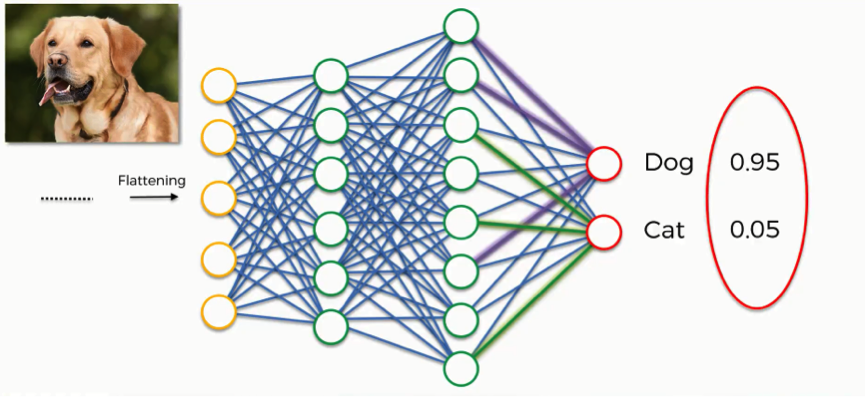
The answer is that they actually don’t coordinate these results together.
The reason that the results have this coherence is that we introduce to the network the first element of this tutorial which is the softmax function.
Softmax
The softmax function goes like this:
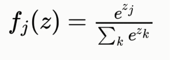

Without this function, the dog and cat classes will each have a real-value probability but the results will not add up to any particular figure.
Right here is Wikipedia’s definition of the softmax function, which is also known as the normalized exponential function:
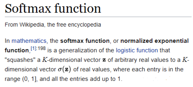
You can forget about all the mathematical jargon in that definition for now, but what we learn from this is that only by including the softmax function are the values of both classes processed and made to add up to 1.
It’s really the only sensible thing to do if you want your convolutional neural network to be of any use.
Otherwise, you would end up in situations where, for example, the probability for the figure in the image being a cat is 90% and 45% for the dog class.
These are virtually useless results.
Cross-Entropy
Hand in hand with the softmax function is the cross-entropy function. Here’s the formula for it:
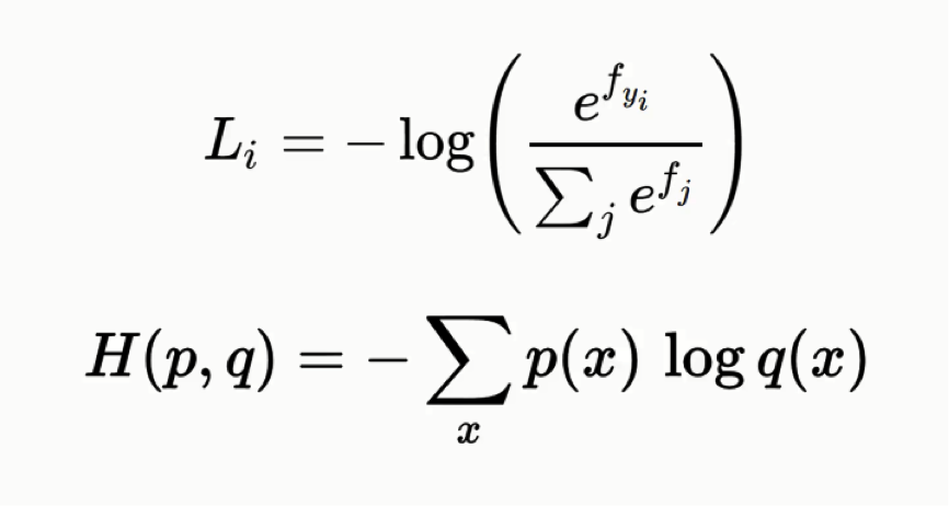
Both formulas are basically equivalent to one another, but in this tutorial, we’ll be using the latter form.
You shouldn’t let the complexity of its name and the formulas overwhelm you, though. The cross-entropy function is actually quite simple as you will see.
If you remember the material from the artificial neural networks section, we had a function called the “mean squared error function.”
We used this function in order to assess the performance of our network, and by working to minimize this mean squared error we would practically be optimizing the network.
The mean squared error function can be used with convolutional neural networks, but an even better option would be applying the cross-entropy function after you had entered the softmax function. Now it’s not called a cost function anymore, but rather a loss function. The differences between the two are not that massive anyway. It’s mainly a terminological difference. You might as well consider them the exact same thing for now.
We will use the loss function in the same manner with which we use the cost function; we’ll try to minimize it as much as possible by optimizing our network.
Demonstration
Let’s look at an example of how this function is used.
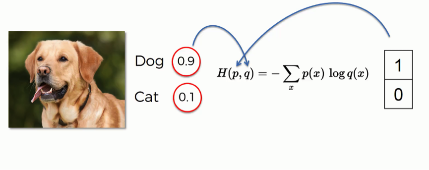
By entering this input image, the network generated a prediction with 90% for the dog class and 10% for the cat.
That provides a “dog” label, hence the 1 and the 0 on the right. When applying the cross-entropy function, you need to make sure that the probabilities on the left go into the “q” slot, and the label values on the right go in the “p” slot. You need to make sure that the order is correct.
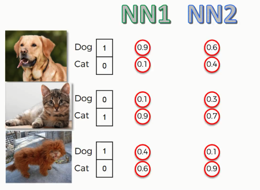
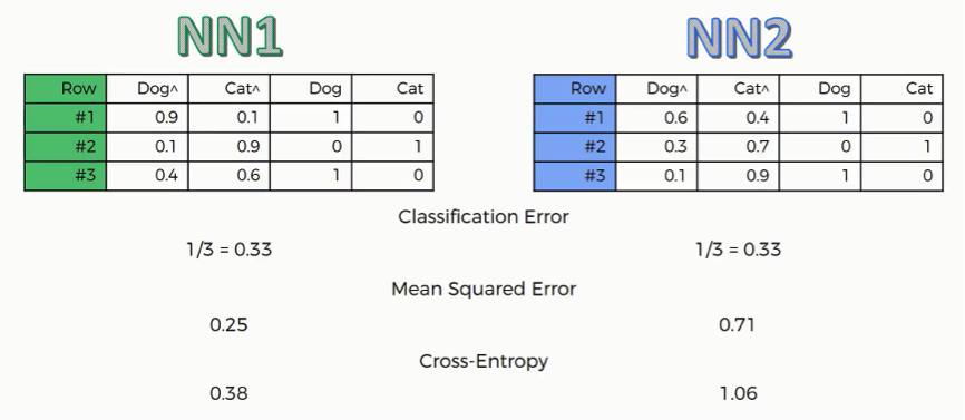
As you can see here, for the first two images, both neural networks came up with similar end predictions, yet the probabilities were calculated with much less accuracy by the second neural network.
For the third image which shows that bizarre lion-looking creature, both neural networks were wrong in their predictions since this animal actually happens to be a dog, but the first neural network was more leaning towards the right prediction than the second one.
So, even when they were both wrong, the second neural network was “more wrong” than the first. What we can do with this data is to try and make an assessment of both network’s performance. To do that, we will have to use one of the functions we mentioned.
First, we’ll need to gather up our data in a table as follows:
Classification Error
This one is very basic. It just tells how many wrong predictions each network made. In our example, each network made one wrong prediction out of three. This function is not all that useful when it comes to backward propagation.
Mean Squared Error
The way you derive the mean squared error is by calculating the squared values of the network’s errors and then get the average of these across the table. In our case, NN2 obviously has a much higher error rate than NN1.
Cross-Entropy
As you can see, the structure of this function’s results differ than the others as we have NN2 with a cross-entropy value of 1.06 and can be somewhat confusing.
Why use the cross-entropy function rather than the mean squared error?
There are several advantages that you get from using the cross-entropy function that are not exactly intuitive or obvious.
We’ll examine here one of the core advantages, and if you want to learn about the remaining reasons for using cross-entropy, you can do so from the material you’ll find mentioned at the end of this tutorial.
At the beginning of your backpropagation process, the output value you have is usually minimal, much smaller than the actual desired value. The gradient is also usually very low, making it difficult for the neural network to actually utilize the data it has in adjusting the weights and optimizing itself.
The cross-entropy function, through its logarithm, allows the network to asses such small errors and work to eliminate them.
Say, the desired output value is 1, but what you currently have is 0.000001. Through some optimization, you are able to make that rise up to 0.001.
When calculating the mean squared error, you subtract one from the other, and thus the change will be too trivial to even consider. When using the cross-entropy function, you take a logarithm before comparing the two values by dividing one by the other.
In this case, the change will turn out to be pretty significant.
In both cases, the degree of change is similar in absolute terms, but in relative terms, the cross-entropy function makes your network much more capable of using this change as its guide in the desired direction, whereas the mean squared error function makes very little use of it.
We can therefore conclude from this that the cross-entropy function is a much more efficient optimization tool.
Note that the cross-entropy function is only that useful with convolutional neural networks, most particularly for purposes of classification. If we’re dealing with a regression problem (artificial neural networks), the mean squared error becomes more preferable.
Additional Material
- As the godfather of deep learning, there’s no one to walk you through the details of softmax and cross-entropy better than Geoffrey Hinton. If you’re interested, you can check out this video where Hinton amazingly breaks down the whole concept.
Apart from this video, you should definitely go through Hinton’s other tutorials. The man has a great way of simplifying things and will help you through various concepts of deep learning with absolute ease.
- You can also check out this blog post from 2016 by Rob DiPietro titled “A Friendly Introduction to Cross-Entropy Loss” where he uses fun and easy-to-grasp examples and analogies to explain cross-entropy with more detail and with very little complex mathematics.
- If you want to get into the heavy mathematical aspects of cross-entropy, you can go to this 2016 post by Peter Roelants titled “How to Implement a Neural Network Intermezzo 2.”
That’s about it with regard to convolutional neural networks.
You have a lot of extra material to sift through, so you can do that if you want to gain more insight on the topics we covered, or else, you can just move to the next section of this deep learning course.
Good luck! That’s it!
Thanks for following this guide on Convolutional Neural Networks, we hope you’ve enjoyed, learned and challenged yourself on this section of Deep Learning A-Z.
It’s step 2 in our journey of Deep Learning. If you liked Convolutional Neural Networks (CNNs) then you’ll be ready for Recurrent Neural Networks.
