

Welcome… To the first step of your Deep Learning adventure. First up, Artificial Neural Networks. Sit back, relax, buckle up and get started with Artificial Neural Networks!
(For the full PPT of Artificial Neural Networks (ANN) Click Here)


Artificial Neural Networks – Plan of Attack
To help you overcome the complexities inherent in Neural Networking, SuperDataScience has developed a seven-stage Plan of Attack, which is hopefully not a precursor to what our creations do when sentience awakens within them.
The Neuron
Building from up from the foundation of the Neural Network we will first examine the Neuron; how it works and what it looks like. It is the centerpiece of the Neural Network. For point of comparison, there will be some examination of the human brain; how that works and why we want to replicate it.
The Activation Function
The next stage will cover The Activation Function. This is the process applied to data within the neuron. We will be exploring which are most commonly used and understanding which is most appropriate for your Neural Network.
Practical Application
Then we get into some deep learning on the machinations of the Neural Network. We will follow one in action to see what we are striving towards. But instead of the T2 slicing open his flesh to reveal the robot skeleton beneath, we’ll be looking at how a Neural Network can predict housing prices. Not as dramatic but potentially just as upsetting.
How Neural Networks Learn
The next three tutorials will focus on what makes Neural Networks so fascinating; how they learn. We will be going into deep learning with the Gradient Descent method. Then we will move on to its refined sibling, the Stochastic Gradient Descent method.
If by this point fiery flashes of Judgement Day have not interrupted your thinking completely, we will have a summary section that covers Backpropagation and how to compile a set of instructions for your Neural Network.
The Neuron
In this deep learning tutorial we are going to examine the Neuron in Neural Networking. Briefly, we will cover:
- What it is
- What it does
- Where it fits in the Neural Network
- Why it is important
The neuron that forms the basis of all Neural Networks is an imitation of what has been observed in the human brain.
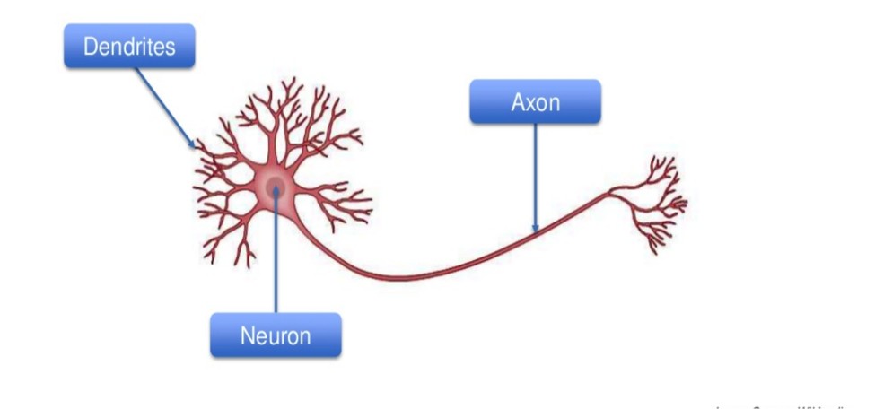
This odd pink critter is just one of the thousands swimming around inside our brains.
Its eyeless head is the neuron. It is connected to other neurons by those tentacles around it called dendrites and by the tails, which are called axons. Through these flow the electrical signals that form our perception of the world around us.
Strangely enough, at the moment a signal is passed between an axon and dendrite, the two don’t actually touch.
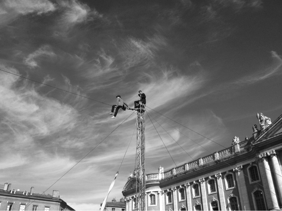
A gap exists between them. To continue its journey, the signal must act like a stuntman jumping across a deep canyon on a dirtbike. This jump process of the signal passing is called the synapse. For simplicity’s sake, this is the term I will also use when referring to the passing of signals in our Neural Networks.
How has the biological neuron been reimagined?
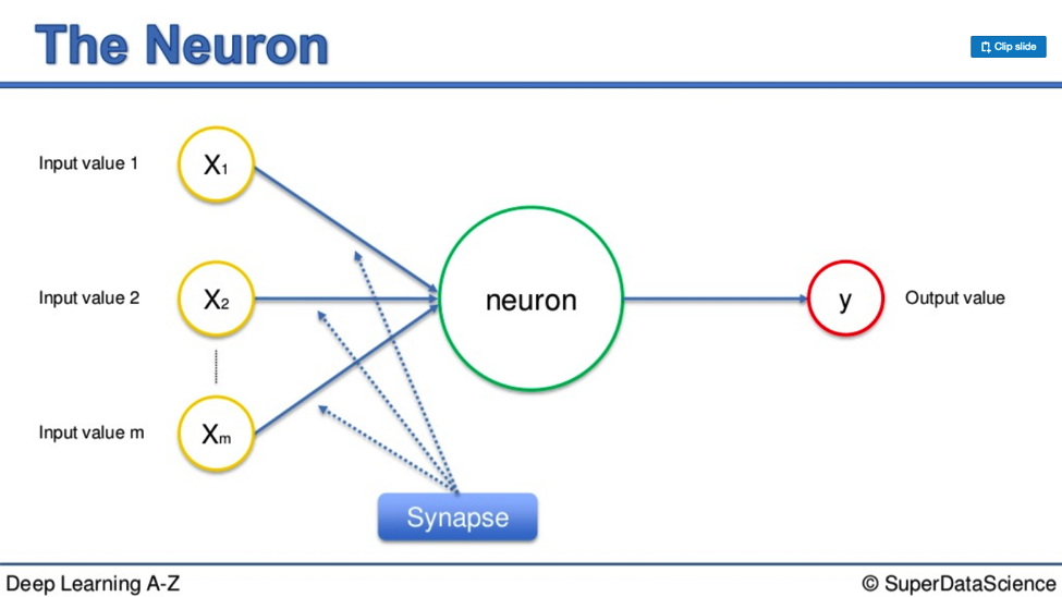
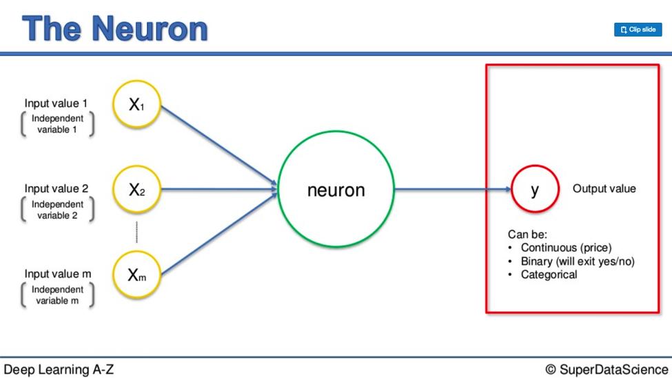
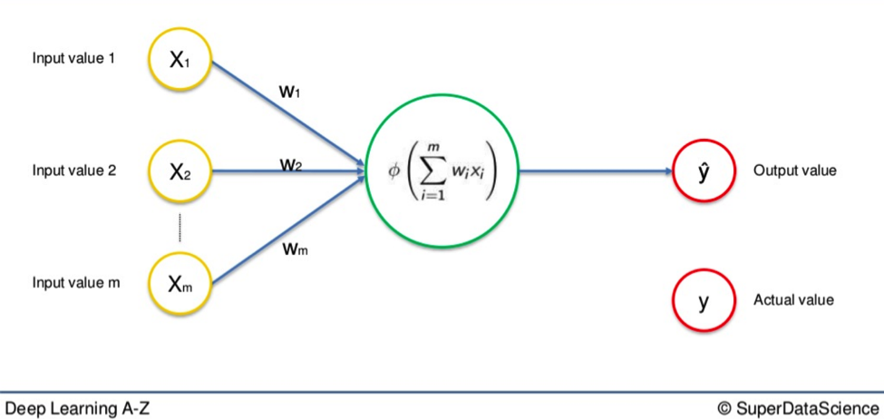
Here is a diagram expressing the form a neuron takes in a Neural Network.
The inputs on the left side represent the incoming signals to the main neuron in the middle. In a human neuron, this these would include smell or touch.
In your Neural Network these inputs are independent variables. They travel down the synapses, go through the big grey circle, then emerge the other side as output values. It is a like-for-like process, for the most part.
The main difference between the biological process and its artificial counterpart is the level of control you exert over the input values; the independent variables on the left-hand side.
You cannot decide how badly something stinks, whether a screeching sound pierces your ears, or how slippery your controller gets after losing, yet again, on FIFA 18.
You can determine what variables will enter your Neural Network
It is important to remember; you must either standardize the values of your independent variables or normalize them. These processes keep your variables within a similar range so it is easier for your Neural Network to process them. This is essential for the operational capacity of your Neural Network.
Observations
It is equally important to note that each variable does not stand alone. They are together as a singular observation. For example, you may list a person’s height, age, and weight. These are three different descriptors, but they pertain to one individual person.
Now, once these values pass through the main neuron and break on through to the other side, they become output values.
Output values
Output values can take different forms. Take a look at this diagram:
They can either be:
- continuous (price)
- binary (yes or no)
- or categorical.
A categorical output will fan out into multiple variables.
However, just as the input variables are different parts of a whole, the same goes for a categorical output.
Picture it like a bobsled team: multiple entities packed inside one vehicle.
Singular Observations
It is important to remember so you can keep things clear in your mind when working through this; both the inputs on the left and the outputs on the right are single observations.
The neuron is sandwiched between two single rows of data. There may be three input variables and one output. It doesn’t matter. They are two single corresponding rows of data. One for one.
Back to the Stuntman
If he’s marauding over the soft pink terrain of the human brain he will eventually reach the canyon we mentioned before. He needs to jump it.
Perhaps there is a crowd of beautiful women and a stockpile of booze on the other side. He can hear ZZ Top blasting from unseen speakers.
He needs to get over there. In the brain, he has to take the leap. He would much rather face this dilemma in a Neural Network, where he doesn’t need the bike to reach his nirvana.
Here, he has a tightrope linking him to the promised land.
This is the synapse.
Weights
Each synapse is assigned a weight.
Just as the tautness of the tightrope is integral to the stuntman’s survival, so is the weight assigned to each synapse for the signal that passes along it.
Weights are a pivotal factor in a Neural Network’s functioning.
Weights are how Neural Networks learn
Based on each weight, the Neural Network decides what information is important, and what isn’t.
The weight determines which signals get passed along or not, or to what extent a signal gets passed along. The weights are what you will adjust through the process of learning. When you are training your Neural Network, not unlike with your body, the work is done with weights.
Later on I will cover Gradient Descent and Backpropagation.
These are concepts that apply to the alteration of weights, the hows, and whys; what works best. That’s everything to do with what goes into the neuron, what comes out, and by what means.
What happens inside the neuron?
How are input signals altered in the neuron so they come out the other side as output signals? I’m sad to say it’s slightly less adventurous than a tiny stuntman taking risks on his travels to who-knows-where.
It all comes down to plain old addition.
First, the neuron takes all the weights it has received and adds them all up. Simple.
It then applies an activation function that has already been applied to either the neuron itself, or an entire layer of neurons. I will go into deeper learning on the activation function later on. For now, all you need to know is that this function facilitates whether a signal gets passed on or not.
That signal goes on to the next neuron down the line then the next, so on and so forth. That’s it.
In conclusion
We have covered:
- Input Values
- Weights
- Synapses
- The Neuron
- The Activation Function
- Output Values
This is the process you will see repeated again and again and again. . . all the way down the line, hundreds or thousands of times depending on the size of your Neural Network and how many neurons are within it.
Additional Reading
For deeper learning on Artificial Neural Networks the Neuron you can read a paper titled Efficient BackProp by Yan LeCun et al. (1998). The link is here.
Join me next time as I cover the activation function and try to invent another imaginary thrill-seeker to illustrate the processes there. Happy learning.
The Activation Function
In this tutorial we are going to examine an important mechanism within the Neural Network: The activation function.
The activation function is something of a mysterious ingredient added to the input ingredients already bubbling in the neuron’s pot.
In the last part of the course we examined the neuron, how it works, and why it is important.
The last section and this one are intrinsically linked because the activation function is the process applied to the weighted input value once it enters the neuron.
Values
If weighted input values are shampoo, floor polish, and gin, the neuron would be the deep black pot. The activation function is the open flame beneath that congeals the concoction into something new; the output value.
Just as you can adjust the size of the flame and time you wish to spend stirring, there are many options you can process your input values with.
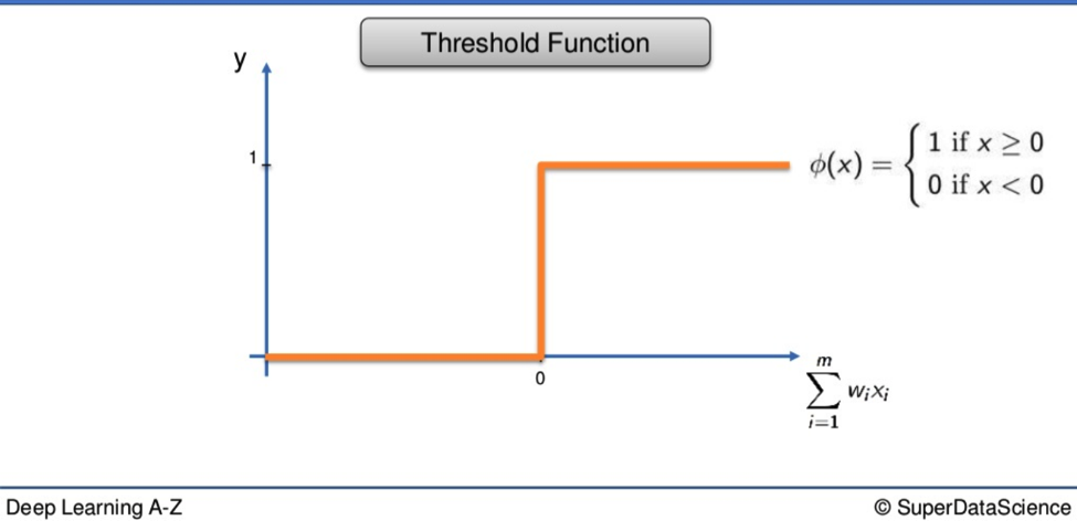
The Threshold Function
The first is the simplest. The x-axis represents the weighted sum of inputs. On the y-axis are the values from 0 to 1. If the weighted sum is valued as less than 0, the TF will pass on the value 0. If the value is equal to or more than 0, the TF passes on 1. It is a yes or no, black or white, binary function.
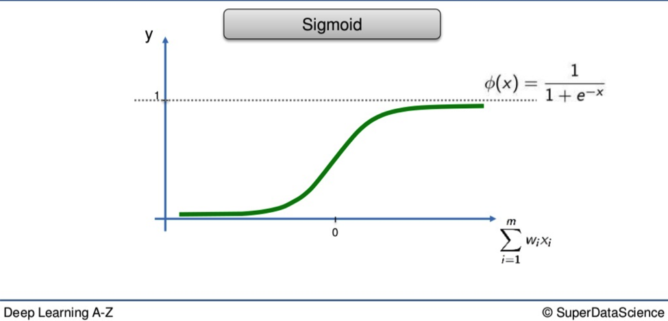
The Sigmoid Function
Here is the second method. With the Sigmoid, anything valued below 0 drops off and everything above 0 is valued as 1.
Shaplier than its rigid cousin, the Sigmoid’s curvature means it is far better suited to probabilities when applied at the output layer of your NN. If the Threshold tells you the difference between 0 and 1 dollar, the Sigmoid gives you that as well as every cent in between.
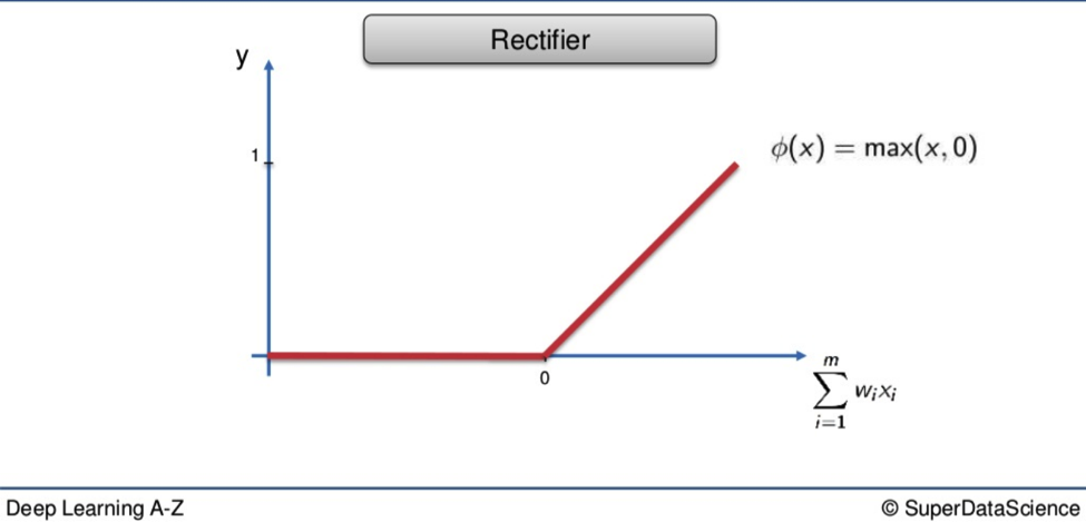
The Rectifier Function
Up next we have one of the most popular functions applied in global Neural Networking today, and with the most medieval name.
You can see why so many people love it.
Look at how the red line presses itself against the x-axis before exploding in a fiery arrow at 45 degrees to a palace above the clouds.
Who wouldn’t want a piece of that sweet action? Its spectacle is matched only by its generosity. Every value is welcome at the party. If a weighted value is below 0 it doesn’t just get abandoned, left to float through time and space between stars and pie signs. It is recruited, indoctrinated. It becomes a 0.
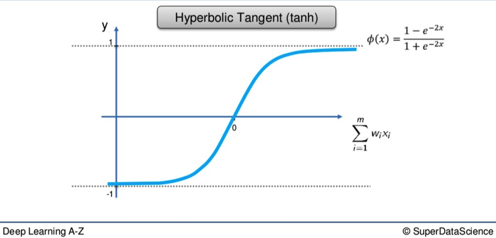
Hyperbolic Tangent Function
Following an act like that was never going to be easy, but the Hyperbolic Tangent Function (tanh), gives it a bloody good go.
Tanh is the Dante of the activation functions.
It is willing to delve deep below the x-axis and its 0 value to the icy pits of the lowest circle, where the value -1 slumbers.
From there it soars on a route similar to that of the Sigmoid, though over a greater span, all the way to blessed 1.
Conclusion
Obviously, this has not been an intensely focused piece on the nuts and bolts of activation functions.
The purpose of this deep learning portion has been to familiarize you with these functions as concepts and to show you the differences between one function and the next.
However, it would be remiss of me to exclude those wanting something more involved.
Additional Reading
I recommend the paper Deep sparse rectifier neural networks by Xavier Glorot et al. (2011). The link is here.
It is not essential you read through such dense material yet. I am more concerned with you applying these functions rather than understanding them absolutely. Once you feel comfortable with the practical applications, then the information in the link above will make more sense.
That’s all for now. I hope it was all easily digestible. In the next section, I will help you understand how Neural Networks work.
How do Neural Networks Work?
Having already looked at the neuron and the activation function, in this tutorial the deep learning begins on how Neural Networks work.
If you have forgotten the structural elements or functionality of Neural Networks, you can always scroll back through the previous articles.
Off the Page and Into Practice
This will be a step-by-step examination of how Neural Networks can be applied by using a real-world example. Property valuations.
The pinnacle of your adult life. The moment you realize the time falling asleep on the couch while watching South Park reruns is finally coming to an end.
You are getting on the property ladder.
Choices, choices
Almost everybody wants to own a house, but I can’t think of anybody who enjoys buying one. Why is that?
Well, it’s time-consuming, boring, and every ill-considered choice can take you a step closer to long-term financial bondage. It’s so stressful. Every option becomes an imperative you must painstakingly consider, and objectively at that. It’s an almost puzzle to solve.
Lucky for us we have Neural Networks. They can find answers quicker than we can and without the hair-tugging vacillation we would likely go through on the way.
Remember
One thing to remember before we get into this example. In this section, we will not be training the network. Training is a very important part of Neural Networking but don’t stress, we will be looking at this later on when we better understand how Neural Networks learn. This part is all about application, so we will imagine our Neural Network is already trained up, primed and ready to go.
Back to the task at hand
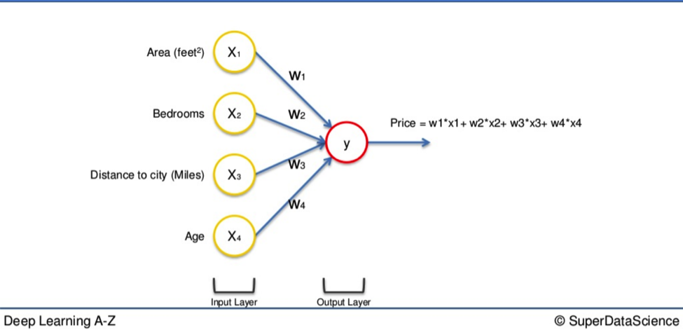
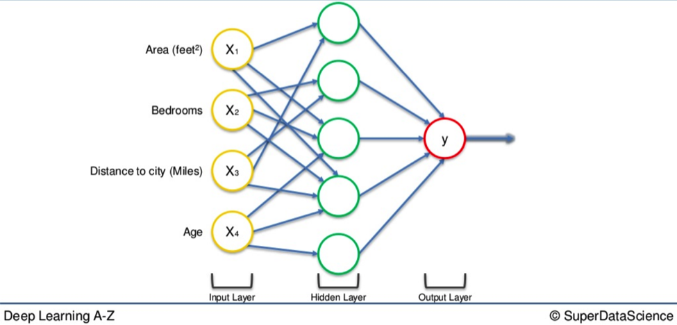
As you will remember, we always begin with a layer of input variables. These are different factors assembled in a single row of data, represented below on the left-hand side.
In this simple example we have four variables:
- Area (feet sq)
- Number of bedrooms
- Distance to city (miles)
- Age of property
Their values go through the weighted synapses straight over to the output layer. All four will be analyzed, an activation function will be applied, and the results will be produced.
This is comprehensive enough on a basic level. But there is a way to amplify the power of the Neural Network and increase its accuracy by a very simple addition to the system.
Power up
You can implement a hidden layer that sits between the input and output layers.
From this new cobweb of arrows, representing the synapses, you begin to understand how these factors, in differing combinations, cast a wider net of possibilities. The result is a far more detailed composite picture of what you are looking for.
Let’s go step-by-step
We begin with the four variables on the left and the top neuron of the hidden layer in the middle. All four variable all be connected to the neuron by synapses.
However, not all of the synapses are weighted. They will either have a 0 value or non 0 value.
The former indicates importance while the latter means they will be discarded.
For instance, the Area and Distance variable may be valued as non 0. Which means they are weighted. This means they matter. The other two variables, Bedrooms and Age, aren’t weighted and so are not considered by that first neuron. Got it? Good.
You may wonder why that first neuron is only considering two of the four variables.
In this case, it is common on the property market that larger homes become cheaper the further they are from the city. That’s a basic fact. So what this neuron may be doing is looking specifically for properties that are large but are not so far from the city.
Properties that, for their proximity to a metropolis, have anomalous amounts of square footage. The benefits of this are clear. A person may have a large family but works and whose children go to school in the city.
It would be beneficial for everybody to have their own space at home and also not to have to wake up when the cock crows every morning.
This is speculation
We have not yet done deep learning on training Neural Networks. Based on the variables at hand this is an educated guess as to how the neuron is processing these variables.
Once the Distance and Area criteria have been met, the neuron applies an activation function and makes its own calculations. These two variables will then contribute to the price in the final output layer.
This is where the power of the Neural Network comes from. There are many of these neurons, each making similar calculations with different combinations of these variables. The next neuron down may have weighted synapses for Area, Bedroom and Age.
It may have been trained up in a specific area or city where there is a high number of families but where many of the properties are new. New properties are often more expensive than old ones.
If you have a new property with three or four bedrooms and large square footage, you can see how the neuron has identified the value of such a place, regardless of its distance to the city.
The way these neurons work and interact means the network itself is extremely flexible, allowing it to look for specific things and therefore make a comprehensive search for whatever it is they have been trained to identify.
That was a simple example of a Neural network in action. In the next tutorial, deep learning on how Neural Networks learn will commence.
How do Neural Networks learn?
Now we have seen Neural Networks in action it is time to get into deep learning on how they learn.
There are two fundamentally different approaches to getting the desired result from your programme.
Hardcoding
This is where you tell the programme specific rules and outcomes, then guide it throughout the entire process, accounting for every possible option the programme will have to deal with. It is a more involved process with more interaction between the programmer and programme.
The other approach is what we have been studying so far.
Neural Networking
With a Network, you create the facility for the programme to understand what it needs to do independently. You provide the inputs, state the desired outputs, and let it work its own way from one to the other.
The difference between these approaches is as follows. Hardcoding is the man driving his car from one point to another, using road signs and a map to navigate his own way to his destination. Neural Networking is a self-driving Tesla.
Let’s revisit some old ground before we plow into fresh earth
Here is a basic Neural Network we have seen many times so far in these tutorials.
You have the single row of input variables on the left.
The arrows that represent weighted synapses go into the large neuron in the middle. And on the right, you have the output value. This is called a Single-Layer Feedforward Neural Network. As you can see, the output value above is represented as Y. This is the actual value.
We are going to replace that with Ŷ, which represents the output value.
The difference between Y and Ŷ is at the core of this entire process.
When input variables go along the synapses and into the neuron, where an activation function is applied, the resulting data is the output value, Ŷ.
In order for our Network to learn we need to compare the output value with the actual value.
There will be a difference between the two.
The Cost Function
Then we apply what is called a cost function (Cost function – Wikipedia), which is one half of the squared difference between the output value and actual value. This is just one commonly used cost function. There are many. We will apply this particular one in our calculations.
The cost function tells us the error in our prediction.
Our aim is to minimize the cost function. The lower the cost function, the closer Ŷ is to Y, and hence, the closer our output value to our actual value.
A lower cost function means higher accuracy for our Network.
Once we have our cost function, a recycling process begins. We feed the resulting data back through the entire Neural Network. The weighted synapses connecting the input variables to the neuron are the only thing we have any control over.
As long as there exists a disparity between Y and Ŷ, we will need to adjust those weights. Once we tweak them a little we run the Network again. A new cost function will be produced, hopefully, smaller than the last.
Rinse and Repeat
We need to repeat this until we scrub the cost function down to as small a number as possible, as close to 0 as it will go.
When the output value and actual value are almost touching we know we have optimal weights and can therefore proceed to the testing phase, or application phase.
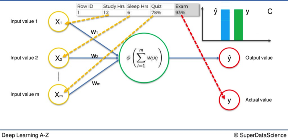
Example
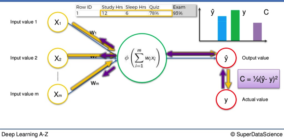
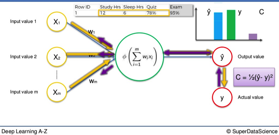
Say we have three input values.
- Hours of study
- Hours of sleep
- Result in a mid-semester quiz
Based on these variables we are trying to calculate the result in an upcoming exam. Let’s say the result of the exam is 93%. That would be our actual value, Y.
We feed the variables through the weighted synapses and the neuron to calculate our output value, Ŷ.
Then the cost function is applied and the data goes in reverse through the Neural Network.
If there is a disparity between Y and Ŷ then the weights will be adjusted and the process can begin all over again. Rinse and repeat until the cost function is minimized.
In this example that would mean our output value would equal the actual value of the 93% test score.
Remember, the input variables do not change.
It is only the weight of the synapses that alters after the cost function comes into play. To give you an idea of the potential scope of this process we can extend this example. The simple Neural Network cited above could be applied to a single student.
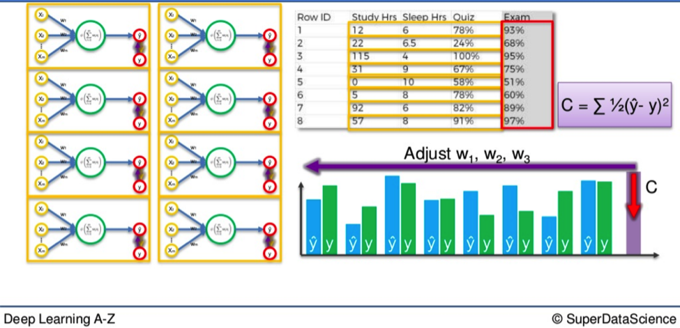
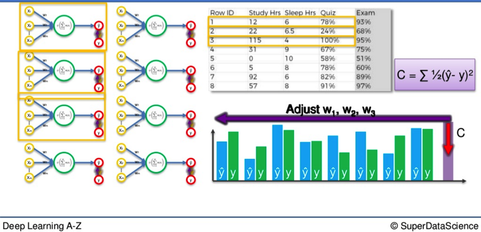
Go Bigger
What if you wanted to apply this process to an entire class? You would simply need to duplicate these smaller Networks and repeat the process again.
However, once you do this you will not have a number of smaller networks processing separately side-by-side.
They actually merge to form a single, much larger Neural Network.
So when you again go through the process of minimizing the difference between Y and Ŷ for an entire class, the cost function phase at the end will adjust for every student simultaneously.
If you have thirty students the Y / Ŷ comparison will occur thirty times in each smaller network but the cost function will be applied to all of them together.
As a result, the weights for every student will be adjusted accordingly, so on and so forth.
Additional Reading
For further reading on this process, I will direct you towards an article named A list of cost functions used in neural networks, alongside applications. CrossValidated (2015).
I hope you found something useful in this deep learning article. See you next time.
Gradient Descent
This is a continuation of the last deep learning section on how Neural Networks learn. If you recall, we summed up the learning process for Neural Networks by focusing on one particular area.
Reducing the Cost Function
The cost function is the difference between the output value produced at the end of the Network and the actual value. The closer these two values, the more accurate our Network, and the happier we are. How do we reduce the cost function?
Backpropagation
This is when you feed the end data back through the Neural Network and then adjust the weighted synapses between the input value and the neuron.
By repeating this cycle and adjusting the weights accordingly, you reduce the cost function.
How do we adjust the weighted synapses?
In the last article, I pointed out that the weights are the only thing within our Network that we can tamper with. Throughout the rest of the process, the Network is essentially operating independently.
This puts all the more emphasis on how and why we alter the weights.
If you make the wrong alteration it would be like having a car with the front axle pointing slightly to the left, and while you are driving you to let go of the steering wheel but keep your foot on the gas.
Sooner or later, you’re going to crash.
Two ways to adjust the weights
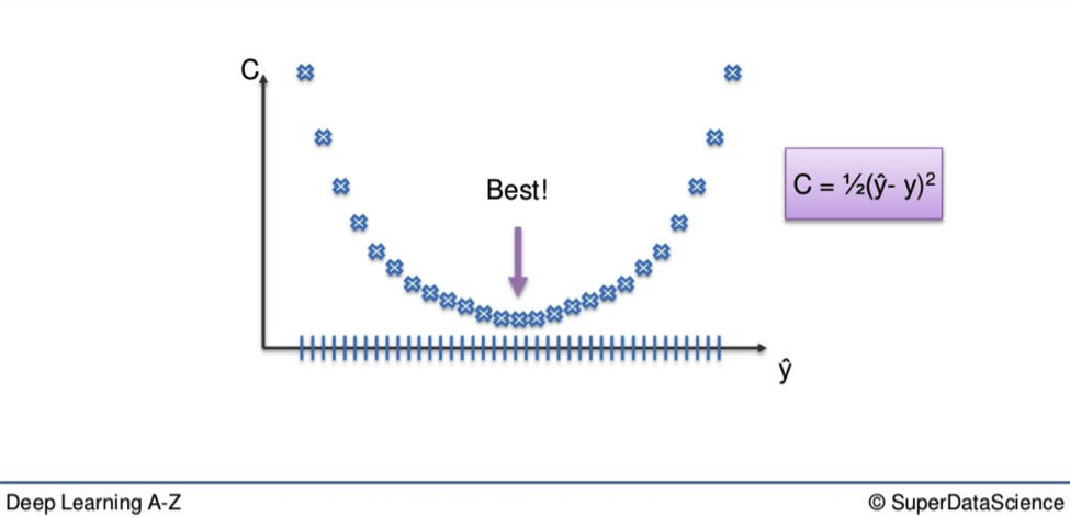
The first is the brute-force approach. This is far better suited to a single-layer feed-forward network. Here you take a number of possible weights. On a graph it looks like this:
You can see there are a number of blue dots. As we have already established, we want to lower the cost function i.e. reduce the difference between our output value and actual values.
We want to eliminate all other weights except for the one right at the bottom of the U-shape, the one closest to 0. The closer to 0, the lower the difference between output value and actual value.
That is where we find our optimal weight.
You could find your way to the best weight through a simple process of elimination. You could trial every weight through your network and one-by-one get closer and closer to your optimal weight. On a simple level, this would suffice, say if you only had a single weight to optimize. But the larger a network becomes, the number of weights that will emerge means this method is impracticable.
You could have an almost infinite amount of weights to adjust. Therefore a process of elimination would be like looking for the prettiest grain of sand on a beach. Good luck with that. This problem is known as the Curse of Dimensionality.
To put a mind-bending timescale on it, an advanced supercomputer would need a longer time than the universe has existed to find all the optimal weights in a mildly complex Neural Network, when using this process of elimination.
Obviously, that won’t do.
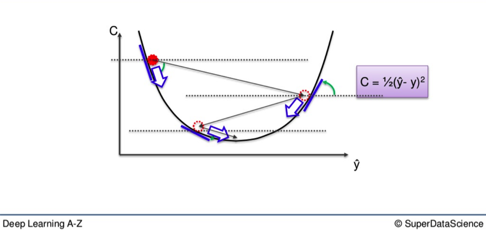
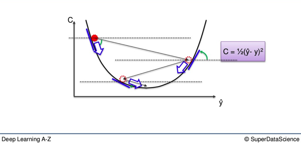
Gradient Descent
Here you see how gradient descent works in a simple graphic representation.
Instead of going through every weight one at a time, and ticking every wrong weight off as you go, you instead look at the angle of the cost function line.
If the slope is negative, like it is from the highest red dot on the above line, that means you must go downhill from there.
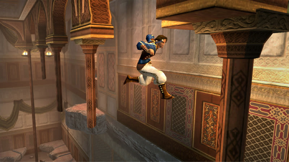
For the sake of remembering the journey downwards, you can picture it like the old Prince of Persia video games.
You need to jump across the open space, from ledge to ledge, until you get to the checkpoint at the bottom of the level, which is our 0.
This eliminates a vast number of incorrect weights on the way down. It also reduces the time and effort spent on finding the right weight.
It is a far more efficient method, I’m sure you will agree. That is just an examination of the process in principle.
At the end of the next section, I will provide you with some additional reading and there will be further information once we reach the application phase.
Next, we will go into deep learning on Stochastic Gradient Descent. See you there.
Stochastic Gradient Descent
This article is the second in a two-parter covering methods by which we can find the optimal weight for our synapses.
Just to remind you, the weights are the only thing we can adjust as we look to bring the difference between our output value and our actual value as close to 0 as possible. This is important because the smaller the difference between those two value, the better our Neural Network is performing.
Gradient Descent
You can see the aforementioned method illustrated in the graph below.
Gradient Descent is a time-saving method with which you are able to leapfrog large chunks of unusable weights by leaping down and across the U-shape on the graph. This is great if the weights you have amassed fit cleanly into this U-shape you see above. This happens when you have one global minimum, the single lowest point of all you weights. However, depending on the cost function you use, your graph will not always plot out so tidily.
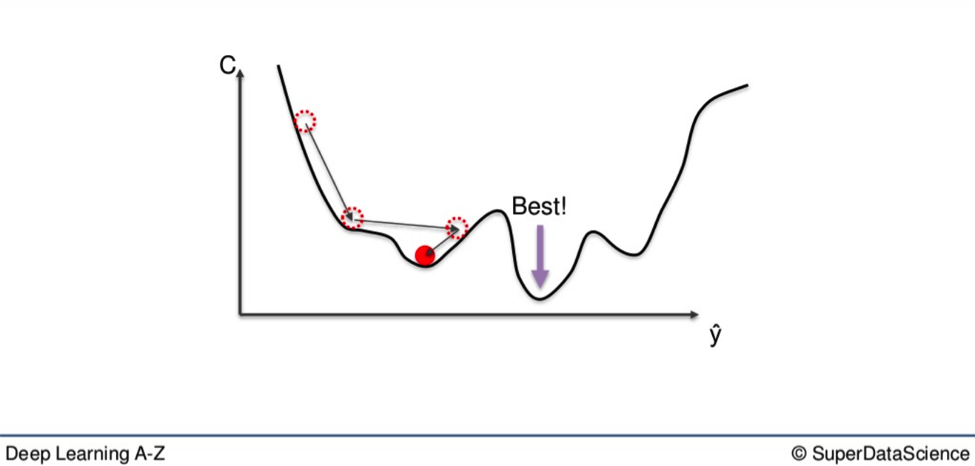
The Difference between Local and Global
If you use the aforementioned Gradient Descent method here, you may very well end up with what is called a local minimum of the cost function.
What you want is the global minimum. See where the red dot is sitting? That is the local minimum. It is a low point on the gradient. But not the lowest. That would be the purple dot, further down.
If you criss-cross down the way you would in the first graph in the article, you may end up stuck at the second-lowest point and never reach optimal weight, which would be the lowest.
For this reason, another method has been developed for when you have a non-convex shape on your graph.
With this, you won’t get bogged down in the nucks higher up on the line before you get to the bottom.
This alternative method is called Stochastic Gradient Descent.
Stochastic Gradient Descent
The difference between Gradient Descent and Stochastic Gradient Descent, aside from the one extra word, lies in how each method adjusts the weights in a Neural Network.
Let’s say we have ten rows of data in our Neural Network.
- We plug them in.
- We calculate our cost function based on whatever formula we happen to be using.
Now, with the Gradient Descent method, all the weights for all ten rows of data are adjusted simultaneously. This is good because it means you start with the same weights across the board every time. The weights move like a flock of birds, all together in the same direction, all the time.
It is a deterministic method.
On the other hand, this can take a little longer than the Stochastic method because with every adjustment, every piece of data has to be loaded up all over again.
With the Stochastic method, each weight is adjusted individually.
So, we go to the first row
- Run the Neural Network.
- Look at the cost function.
- Then we adjust the weights.
Then we go to the second row
- Run the Neural Network.
- Look at the cost function.
- Adjust the weights.
Row after row we do this until all ten rows have been run through.
The Stochastic method is a lighter algorithm and therefore faster than its all-encompassing cousin.
It also has much higher fluctuations, so on a non-convex graph it is more likely to find the global minimum rather than the local minimum. There is a hybrid of these two approaches called the Mini-Batch method.
Mini-batch method
With this, you don’t have to either run one row at a time or every row at once. If you have a hundred rows of data you can do five or ten at a time, then update your weights after every subsection has been run.
Additional Reading
There is some additional reading available for this section. I recommend A Neural Network in 13 Lines of Python (Part 2 – Gradient Descent) by Andrew Trask (2015). The link is here.
There is also a book called Neural Networks and Deep Learning by Michael Nielsen (2015).
That is the nutshell version of the differences between Gradient Descent and Stochastic Gradient Descent. Our next and final section will cover Backpropagation. See you there.
Backpropagation
Unfortunately friends, this is our final deep learning tutorial.
But fear not, before the tears begin to flow too freely, you can stem the tide with some lovely, soft Backpropagation.
Adjusting
Backpropagation is an advanced algorithm, driven by sophisticated mathematics, which allows us to adjust all the weights in our Neural Network.
This is important because it is through the manipulation of weights that we bring the output value (the value produced by our Neural Network) and the actual value closer together.
These two values need to be as close as possible.
If they are far apart we use Backpropagation to run the data in reverse through the Neural Network. The weights get adjusted. Consequently, we are brought closer to the actual value.
In a Nutshell
The key underlying principle of Backpropagation is that the structure of the algorithm allows for large numbers of weights to be adjusted simultaneously.
This drastically speeds up the process and is a key ingredient as to why Neural Networks are able to function as well as they do.
Additional Reading
I mentioned this in the last post but I will include some additional reading material in case you want to get into some extra deep learning on this process. Neural Networks and Deep Learning by Michael Nielsen (2015) is all you will need to go full Einstein on this subject. Give it a look.
Several times throughout this course I have mentioned the importance of training your Neural Network. I wanted you to see the Networks in action before examining how they operate, I have left this until last.
A step-by-step training guide for your Neural Network
- Randomly initialize the weights to small numbers close to 0 (but not 0).
- Input the first observation. One feature per input node.
- Forward-Propagation. From left to right the neurons are activated and the output value is produced.
- Compare output value to actual value. Measure the difference between the two; the generated error.
- From right to left the generated error is back-propagated and the weights adjusted accordingly. The learning rate of the Network is dependent on how much you adjust the weights.
- Repeat steps 1-5 and either adjust the weights after each observation (Reinforcement learning), or after a batch of observations (Batch learning).
- When the whole training set passes through the Neural Network, that makes an epoch. Redo more epochs.
And that is that. I hope this deep learning experience has been somewhat useful to you. I hope you come back soon.