

How do Self-Organizing Maps Learn? (Part 2)
(For the PPT of this lecture Click Here)
Let’s move to the second part of our tutorial on how SOMs learn. Like we said at the end of our last tutorial, this time we’ll be examining the SOM learning process at a more sophisticated level. Our map this time will contain multiple best-matching units (BMUs) instead of just two.
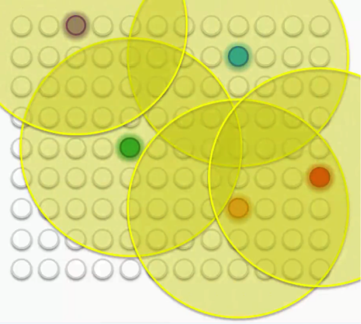
We mentioned in our last tutorial how the BMUs will have to have their weights updated in order to be drawn closer to the data points. Then each of these BMUs will be assigned a radius like in the image below.
Let’s examine these BMUs one by one.
Take the purple node at the top-left. It has been updated so as to be brought closer to the row with which it matches up. The other nodes that fall into its radius undergo the same updates so that they’re dragged along with it. The same goes for each of the other BMUs along with the nodes in their peripheries.
Of course, in that process, the peripheral nodes are going through some push and pull since many of them fall within the radii of more than one BMU. They are updated by the combine forces of these BMUs, with the nearest BMU being the most influential.
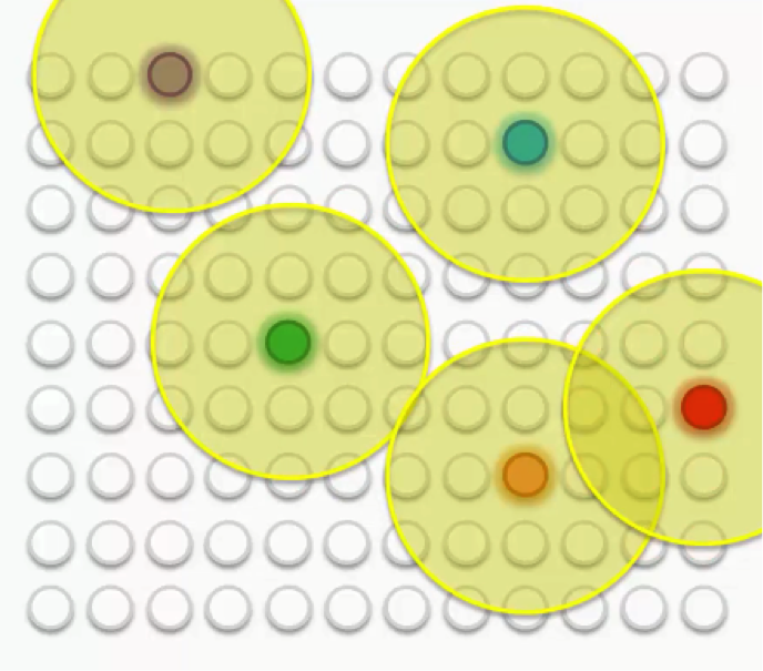
As we repeat this process going forward, the radius for each BMU shrinks. That’s a unique feature of the Kohonen algorithm. That means that each BMU will start exerting pressure on fewer nodes.
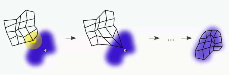
As we proceed, we move from trying to merely let our BMUs touch the data points to trying to align the entire map with the dataset with more precision.
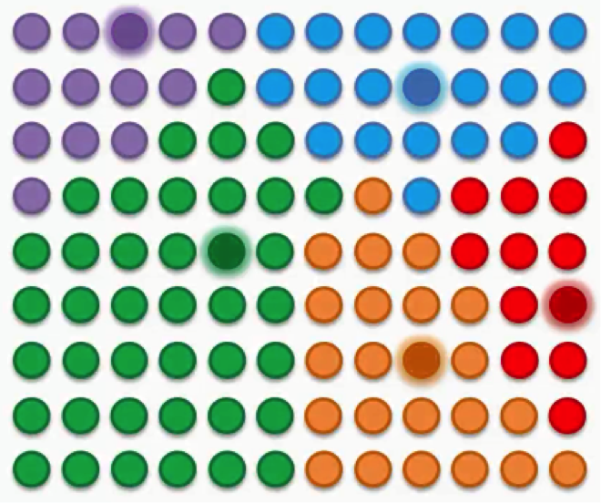
In visual terms, that would lead us to a map that looks something like this:
After all the push and pull between the nodes and the different BMUs, we have come to a point where each node has been assigned a BMU.
There are a few points to bear in mind here:
- SOMs retain the interrelations and structure of the input dataset.
The SOM goes through this whole process precisely to get as close as possible to the dataset. In order to do that, it has to adopt the dataset’s topology.
- SOMs uncover correlations that wouldn’t be otherwise easily identifiable.
If you have a dataset with hundreds or thousands of columns, it would be virtually impossible to draw up the correlations between all of that data. SOMs handle this by analyzing the entire dataset and actually mapping it out for you to easily read.
- SOMs categorize data without the need for supervision.
As we mentioned in our introduction to the SOM section, self-organizing maps are an unsupervised form of deep learning. You do not need to provide your map with labels for the categories for it to classify the data.
It develops its own classes.
- SOMs do not require target vectors nor do they undergo a process of backpropagation.
If you remember from our artificial neural networks section, the network would need to be provided with a target vector (supervision). The data then goes through the network, extract results, compare them to the target vector, detect any errors, and then backpropagate these findings in order to update the weights.
Since we have no target vector, seeing as how SOMs are unsupervised, there would consequently be no errors for the map to backpropagate.
- There are lateral connections between output nodes.
The only connection that emerges between the output nodes in an SOM is the push-and-pull connection between the nodes and the BMUs based on the radius around each BMU. There is no activation function as with artificial neural networks.
You will sometimes see the nodes lined up in a grid, but the only function for that grid is to clarify that these nodes are part of an SOM and to neatly organize them. The grid does not connect the nodes.
Additional Readings
If you’re interested in a slightly deeper introduction to SOMs, you can read this post from 2004 by Mat Buckland. The post covers some of the math behind SOMs, which is quite straightforward compared to some of the mathematical operations that are used when dealing with neural networks.
He also breaks down in more detail the process by which nodes line up into the radii, how BMUs are drawn closer to the data points, etc.
We’re now done with the theoretical part of the SOM section. In our next tutorial we’ll go together through a live example that demonstrates what we learned.