

How do Self-Organizing Maps Learn? (Part 1)
(For the PPT of this lecture Click Here)
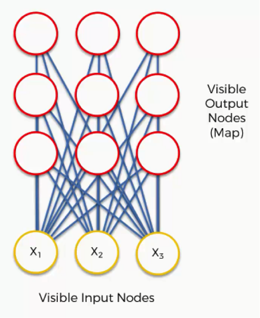

Now it’s time for us to learn how SOMs learn. Are you ready? Let’s begin. Right here we have a very basic self-organizing map.
Our input vectors amount to three features, and we have nine output nodes. If you remember the earlier tutorials in this section, we said that SOMs are aimed at reducing the dimensionality of your dataset.
That being said, it might confuse you to see how this example shows three input nodes producing nine output nodes. Don’t get puzzled by that.
The three input nodes represent three columns (dimensions) in the dataset, but each of these columns can contain thousands of rows. The output nodes in an SOM are always two-dimensional.
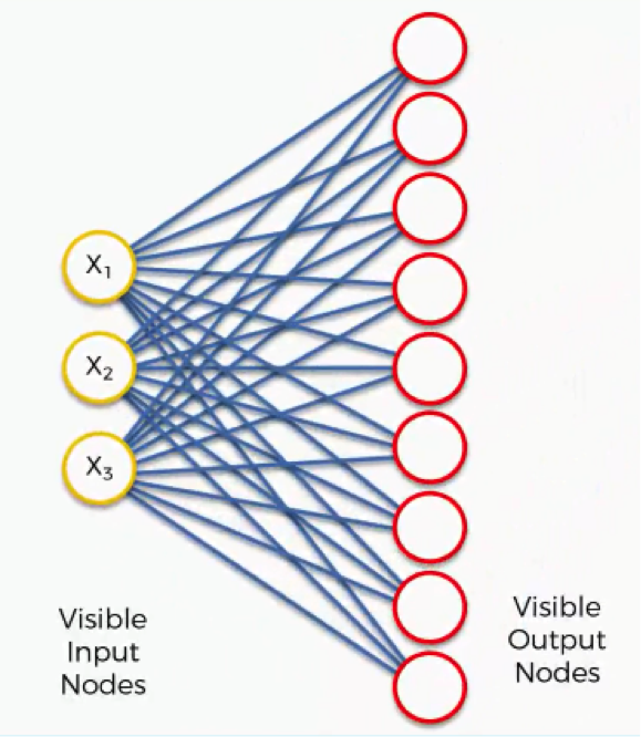
Now what we’ll do is turn this SOM into an input set that would be more familiar to you from when we discussed the supervised machine learning methods (artificial, convolutional, and recurrent neural networks) in earlier sections.
Here’s what it would look like.
It’s still the exact same network yet with different positioning of the nodes. It contains the same connections between the input and the output nodes.
There are, however, differences in the SOMs from what we learned about the supervised types of neural networks:
- SOMs are much simpler.
- Because of their being different, some of the terms and concepts (e.g. weights, synapses, etc.) that we learned in earlier sections will carry different meanings in the context of SOMs. Try not to get confused by these terms.
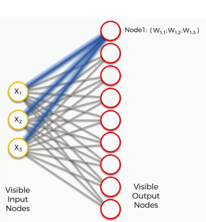
Now, let’s take the topmost output node and focus on its connections with the input nodes. As you can see, there is a weight assigned to each of these connections.
Again, the word “weight” here carries a whole other meaning than it did with artificial and convolutional neural networks. For instance, with artificial neural networks we multiplied the input node’s value by the weight and, finally, applied an activation function. With SOMs, on the other hand, there is no activation function.
Weights are not separate from the nodes here. In an SOM, the weights belong to the output node itself. Instead of being the result of adding up the weights, the output node in an SOM contains the weights as its coordinates. Carrying these weights, it sneakily tries to find its way into the input space.
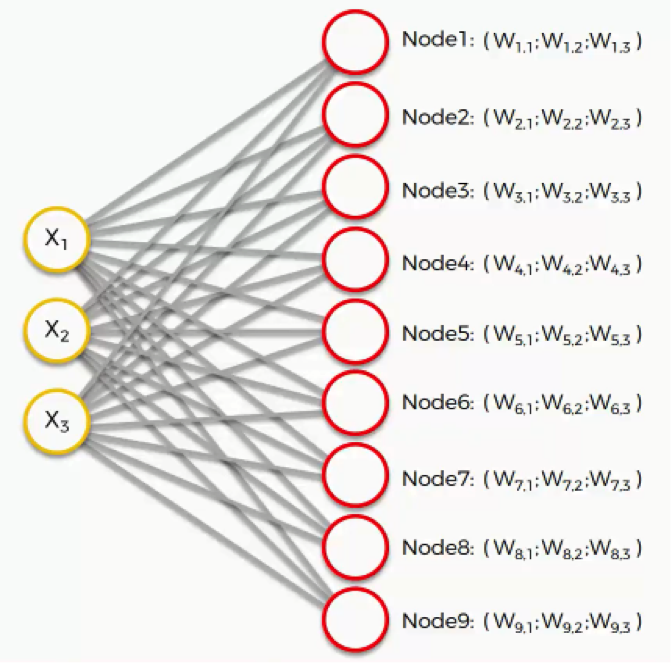
In this example, we have a 3D dataset, and each of the input nodes represents an x-coordinate. The SOM would compress these into a single output node that carries three weights. If we happen to deal with a 20-dimensional dataset, the output node in this case would carry 20 weight coordinates.
Each of these output nodes do not exactly become parts of the input space, but try to integrate into it nevertheless, developing imaginary places for themselves.
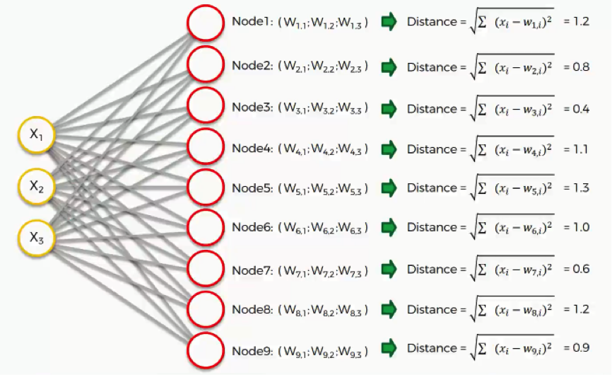
The next step is to go through our dataset. For each of the rows in our dataset, we’ll try to find the node closest to it. Say we take row number 1, and we extract its value for each of the three columns we have. We’ll then want to find which of our output nodes is closest to that row.
To do that, we’ll use the following equation.
As we can see, node number 3 is the closest with a distance of 0.4. We will call this node our BMU (best-matching unit).
What happens next?
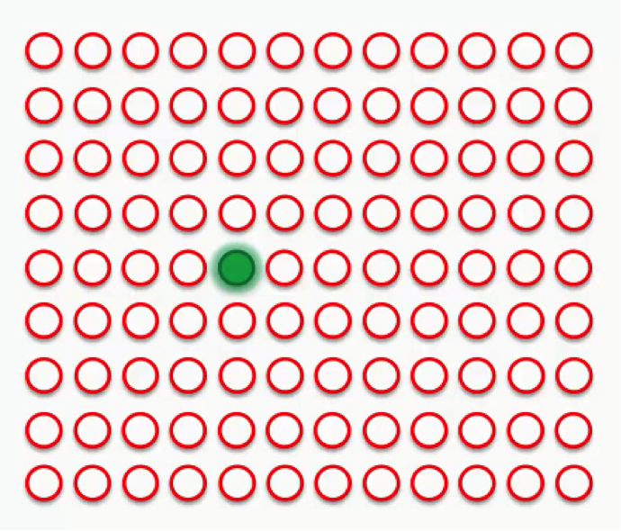
To understand this next part, we’ll need to use a larger SOM.
Supposedly you now understand what the difference is between weights in the SOM context as opposed to the one we were used to when dealing with supervised machine learning. The green circle in the figure above represents this map’s BMU.
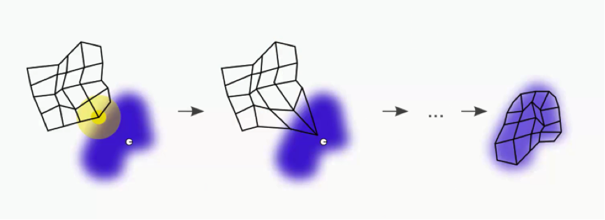
Now, the new SOM will have to update its weights so that it is even closer to our dataset’s first row. The reason we need this is that our input nodes cannot be updated, whereas we have control over our output nodes.
In simple terms, our SOM is drawing closer to the data point by stretching the BMU towards it. The end goal is to have our map as aligned with the dataset as we see in the image on the far right.
That’s a long process, though. Right now we only care about that BMU. As you can see in the first image, the BMU (yellow circle) is the closest to the data point (the small white circle). As you can also see, as we drag the BMU closer to the data point, the nearby nodes are also pulled closer to that point.
Our next step would be to draw a radius around the BMU, and any node that falls into that radius would have its weight updated to have it pulled closer to the data point (row) that we have matched up with.
The closer a node is to the BMU, the heavier the weight that will be added to in its update.
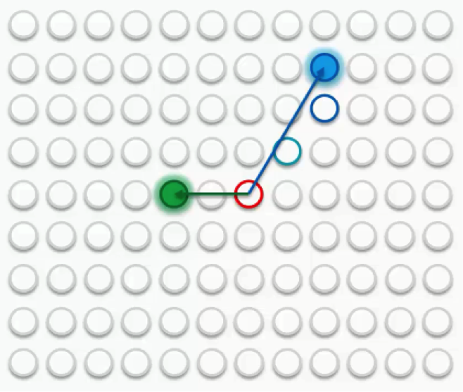
If we then choose another row to match up with, we’ll get a different BMU. We’ll then repeat the same process with that new BMU.
Sometimes a node will fall into both radii, the one drawn around the green BMU as well as the one around the blue BMU. In this case, the node will be affected more by its nearest BMU, although it would still be affected at a lesser degree by the further one.
If, however, the node is almost equidistant from both BMUs, its weight update would come from a combination of both forces.
This should clarify for you how a self-organizing map comes to actually organize itself. The process is quite simple as you can see. The trick is in its repetition over and over again until we reach a point where the output nodes completely match the dataset.
In the next tutorial, we’ll get to see what happens when a more complex output set with more BMUs has to go through that same process. We’ll see you in the next tutorial!