

EXTRA: K-means Clustering (Part 3)
(For the PPT of this lecture Click Here)


So far we have tried out multiple examples on the K-means process and in the last tutorial we introduced K-means++ as a way to counter the random initialization trap. In all these cases, we were working with predetermined numbers of clusters. The question that we’ll try to answer in this tutorial is: How do we decide the right number of clusters in the first place?
There’s an algorithm that specifically performs this function for us, and that’s what we’ll be discussing here. Again, we’ll start right away with an example. Here we have a scatter plot representing a dataset where we have two variables, x and y.
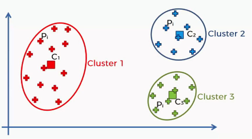
By applying the K-means algorithm to this dataset with the number of clusters predetermined at 3, we would end up with the following outcome.
Keep in mind that the K-means++ had to be implemented in order for us to avoid the Random Initialization Trap. As we mentioned in the previous tutorial, though, you do not need to concern yourself with how that happens at the moment.
Now we want to know the metric or the standard that we can refer to when trying to come up with the “right” number of clusters.
Are 3 clusters enough? Or are 2 just enough? Or perhaps we need 10 clusters?
More importantly, what are the possible outcomes that each of these scenarios can leave us with?
In comes the WCSS.
Within Cluster Sum of Squares (WCSS)
That might look a bit confusing to you, but there’s no need for panicking. It’s simpler than you think. Here’s a quick breakdown of the WCSS. Each of the elements in this algorithm is concerned with a single cluster. Let’s take the first cluster.
What this equation signifies is this: For Cluster 1, we’ll take every point (Pi) that falls within the cluster, and calculate the distance between that point and the centroid (C1) for Cluster 1. We then square these distances and, finally, calculate the sum of all the squared distances for that cluster. The same is done for all the other clusters.
How does this help us in knowing what number of clusters we should use? That’s our next point.
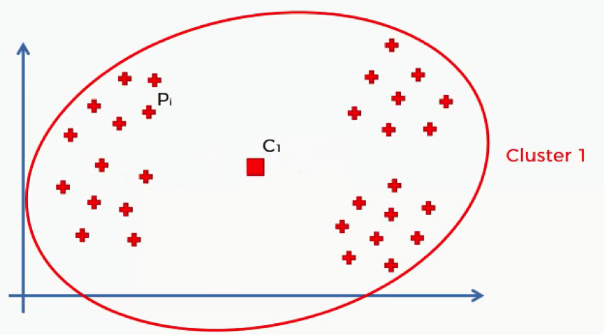
Let’s take an example that we previously discussed where we have a single cluster. We’ll see, roughly, what results that will give us when put through the WCSS algorithm and how that would change as we add more clusters.
Of course, with that many data points inside a single cluster and given their wide distances from the cluster’s centroid, we’ll inevitably end up with a fairly large sum.
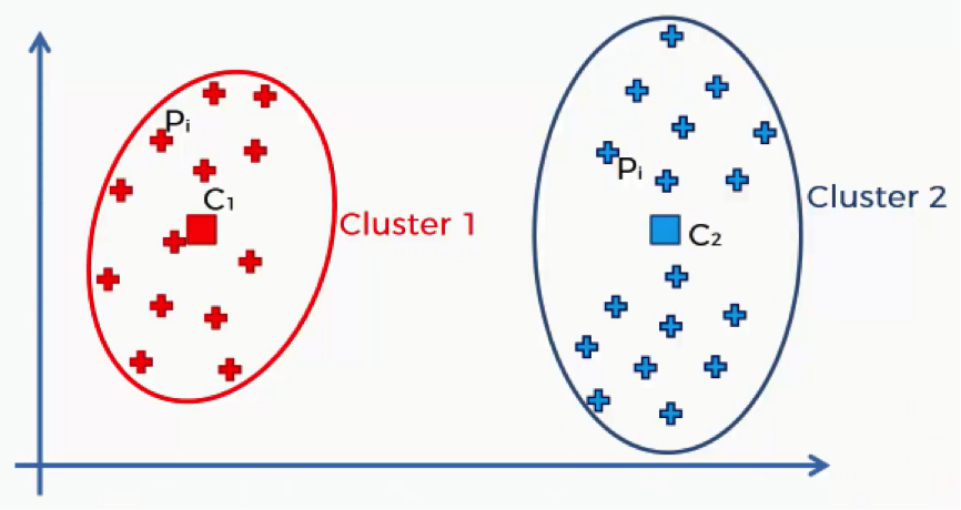
Let’s split up that same scatter plot into two clusters and see what happens.
As you can see, now that we have more clusters, each data point will find itself nearer to its centroid. That way the distances, and consequently the sum of squared distances, will become smaller than when we had a single centroid.
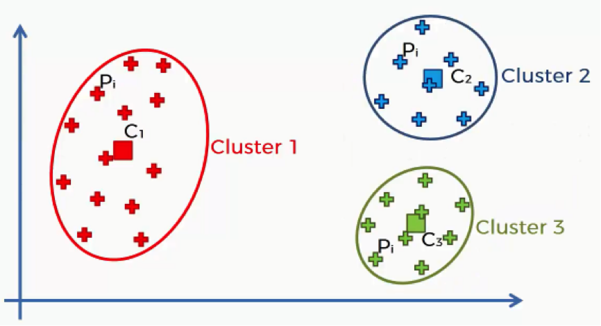
Now, let’s step it up another cluster.
The cluster on the left did not change at all, and so the sum of its squared distances will remain unchanged as well.
The cluster that was on the right in the previous step has now been split up into two clusters, though. That means that each data point has moved even closer to its centroid. That means that the overall sum will again decrease.
Now that you get the idea, we can ask the question of “how far can our WCSS keep on decreasing?”
Our limit is to have one cluster for each data point. You just can’t have 21 clusters for 20 data points. You need each point to be matched up with one centroid.
You can now take a moment to think of what would happen to the WCSS results if we created a cluster for each point. If you said to yourself that you would end up with ZERO then you are absolutely right.
If each point has its own centroid, then that means that the centroid will be exactly where the point is. That, in turn, would give us a zero distance between each data point and its centroid, and as we all (hopefully) know, the sum of many zeros is a zero.
As the WCSS decreases with every increase in the number of clusters, the data points become better fit for their clusters.
So, do we just keep working towards smaller WCSS results or is there a point before the zero level which we can consider optimal?
This next graph can help us answer this question.
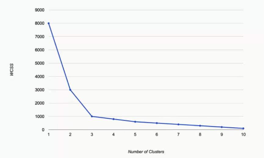
What we have here are the WCSS results as we incrementally increase the number of clusters in a dataset.
You can see that as we move from one cluster to two, the WCSS takes a massive fall from 8,000 to 3,000. It’s unimportant to think of the significance of these numbers at the moment. Let’s just focus on the degrees of change.
As we move from two to three, the WCSS still decreases substantially, from 3,000 to 1,000. From that point on, however, the changes become very minimal, with each cluster only shaving off 200 WCSS points or less.
That’s our hint when it comes to choosing our optimal number of clusters. The keyword is: Elbow.
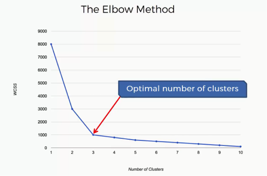
The Elbow Method
What is meant by the “Elbow Method” is looking for the point on this graph where the last substantial change has occurred and the remaining changes are insignificant. In this case, we reach that point at 3 clusters.
If you look at the curve at 3, you will see an elbow shape.
Of course, the “elbow” in your graph will not always be as obvious as in this example. You’re likely to have situations where each person would choose a different point, each thinking that theirs is the optimal point.
That’s where you have to make your judgment call as a data scientist. The Elbow Method can only give you a hint at where to look.
By now you have all the knowledge you need about K-means clustering to move on to the next step.
We’ve set up some exciting challenges that will give you all the practice you need to master K-means clustering using various languages.
Get ready to conquer this topic once and for all!