Self Organizing Maps (SOM’s) – EXTRA: K-means Clustering (part 2)

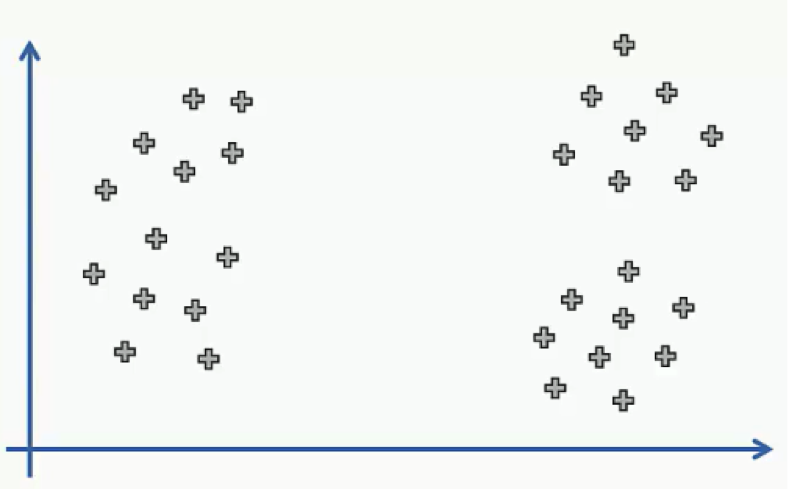
This time we’ll focus on a very specific part of the K-means algorithm; the Random Initialization Trap. Let’s start right off the bat with an example that will demonstrate what the random initialization trap actually is. Here’s a scatter plot with two variables (x and y).

Let’s say we’ve decided to divide our data points into three clusters.

Intuitively, you can probably look at that scatter plot and guess how the three clusters are going to be lined up and which group of data points will fall into each cluster.

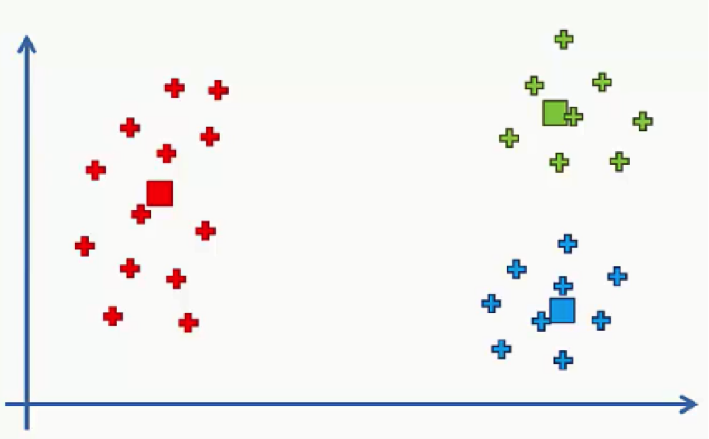
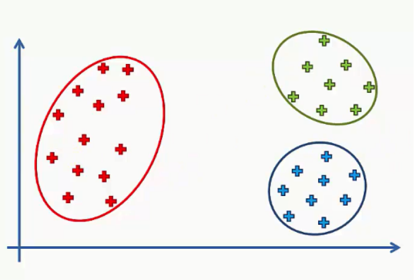
After determining our centroids, assigning each centroid its data points, and performing the rest of the K-means algorithm, we would end up with the following three clusters.

The question here is whether we can change the results and end up with different clusters if we changed the positions of our centroids.

Of course, what we expect from this algorithm is to provide us with proper results, not ones that we can manipulate by playing around with the centroids.

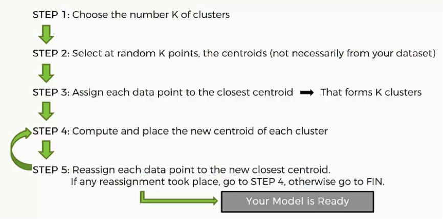
In case you’re confused as to what defines a good or a bad random initialization, just know that we’re using the term “bad” in the loosest sense possible. Let’s go through a quick recap of the K-means process.

As you can see, the entire process is dependent on the first two steps which you are responsible to arbitrarily decide. After you choose the centroids, the rest of the algorithm becomes more deterministic.

Now, let’s try to change our centroids in the second step and see how the rest of the algorithm will play out.

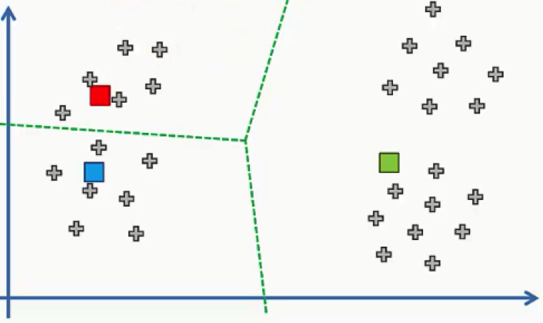
Here are our new centroids, and just to make things easier on ourselves, we can use the same equidistant lines that we used in part 1 on K-means clustering.

These lines will help us assign data points to their nearest centroids more efficiently.

We’ll then move on to step 4 where we compute and place the new centroids. This action is supposed to be done over and over again until there are no reassignments of data points to be made.

You can obviously see the difference between these clusters and the ones we had at the beginning of our example.

If you look at the clusters below, which were gathered around our original centroids, as we said earlier, you can intuitively detect the patterns before the assignment of the data points to centroids was actually made.

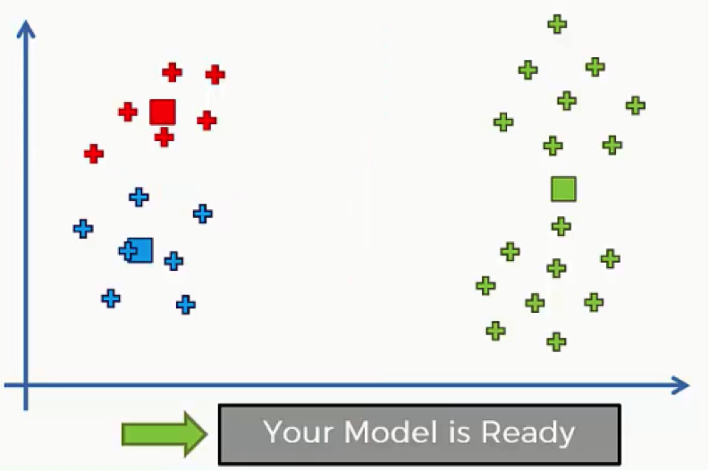
That’s the difference between the two situations. The new centroids with the clusters formed around them are not exactly “intuitively detectable.” You wouldn’t look at the scatter plot and imagine these as the clusters that you will end up with.

Here’s a prime example of how your initialization of the K-means operation can impact the results in a major way. That’s what is known as the Random Initialization Trap.

K-Means++

There’s a remedy for this problem that is used as a supplement to the K-means algorithm. It’s called the K-means++. We won’t discuss this algorithm or its structure in depth, but you only need to know for now that it is hugely beneficial in solving this initialization problem.

Here’s a link to the K-means++ page on Wikipedia. You can do some additional reading about the topic on your own.

The good news is that you don’t need to implement the K-means++ algorithm yourself. Whether you’re using R or Python in the process, the K-means++ is implemented in the background.

You only need to make sure that you are using the right tools in creating your K-means clusters and the correction will be automatically taken care of.

It’s a useful thing to understand nevertheless. It helps you understand the fact that, despite the random selection, there is a specific “correct” cluster that you’re searching for, and that the other clusters that can emerge might be wrong.

They can at least be “undesirable.” That’s it for this part, and as we said, it can do you some good to read about K-means++ as an introduction to what goes on underneath the hood.

Continue with Self Organizing Maps (SOM’s) – EXTRA: K-means Clustering (Part 2) by Clicking Here