

Simple Linear Regression: Step 2
(For the PPT of this lecture Click Here)

As we said in the last tutorial on simple linear regression intuition, the simple regression line in a nutshell is a trend line that best fits your data. We said that in this tutorial we will be discussing what that really means.
It’s quite a brief tutorial.
Are you ready?
The “Best Fitting” Line
So, how does the simple linear regression equation help you find that “best fitting” line we’re talking about?
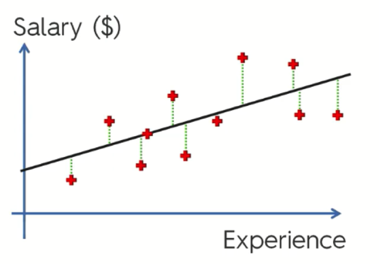
Let’s take another look at the salary-experience example from the last tutorial.
As you can see, we have the observation data plotted all over the graph, as well as the simple regression line running through its points.
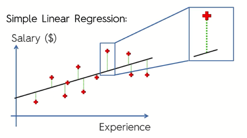
Now, let’s pick a random point and examine it more closely.
Here we have the salary of someone with x years of experience. The straight line represents where that person’s salary should be according to our simple linear regression model, whereas the red point is what that person is actually earning.
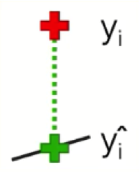
Typically, these two corresponding points are named as shown in this figure below.
The difference between the two is the gap between our observation and our model.
What you do with these points is measure the green line connecting them together. That is the value of the gap. You do the same with each two corresponding points on the graph, square them, and then, finally, sum them up.
After calculating the sum, you then find the minimum value.
The Wrap-Up
So, what the simple linear regression process does is help us draw all of the possible lines using a set of data, and then by calculating the sum of their squares with every single line and recording it, it is able to detect the minimum sum of squares.
The line with the minimum sum of squares possible is the best fitting line.