

Long Short Term Memory – (LSTM)
Long short-term memory (LSTM) network is the most popular solution to the vanishing gradient problem. Are you ready to learn how we can elegantly remove the major roadblock to the use of Recurrent Neural Networks (RNNs)?
Here is our plan of attack for this challenging deep learning topic:
- First of all, we are going to look at a bit of history: what LSTM came from, what was the main idea behind it, why people invented it.
- Then, we will present the LSTM architecture.
- And finally, we’re going to have an example walkthrough.
Let’s get started!
Refresh on the Vanishing Gradient Problem
LSTMs were created to deal with the vanishing gradient problem. So, let’s have a brief reminder on this issue.
As we propagate the error through the network, it has to go through the unraveled temporal loop – the hidden layers connected to themselves in time by the means of weights wrec. Because this weight is applied many-many times on top of itself, that causes the gradient to decline rapidly.
As a result, weights of the layers on the very far left are updated much slower than the weights of the layers on the far right. This creates a domino effect because the weights of the far-left layers define the inputs to the far-right layers. Therefore, the whole training of the network suffers, and that is called the problem of the vanishing gradient.
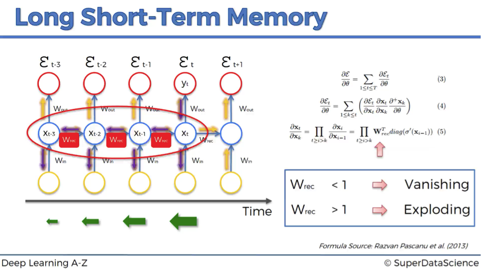
We’ve also defined that as a rule of thumb, if wrec is small – the gradient is vanishing, and if wrec is large – the gradient is exploding.
But what’s “large” and “small” in this context? In fact, we can say that we have a vanishing gradient if wrec < 1 and exploding gradient if wrec > 1. Then, what’s the first thing that comes to your mind to solve this problem?
Probably, the easiest and fastest solution will be to make wrec = 1. That’s exactly what was done in LSTMs. Of course, this is a very simplified explanation, but in general, making recurrent weight equal to one is the main idea behind LSTMs.
Now, let’s dig deeper into the architecture of LSTMs.
LSTM architecture
Long short-term memory network was first introduced in 1997 by Sepp Hochreiter and his supervisor for a Ph.D. thesis Jurgen Schmidhuber. It suggests a very elegant solution to the vanishing gradient problem.
Overview
To provide you with the most simple and understandable illustrations of LSTM networks, we are going to use images created by Christopher Olah for his blog post, where he does an amazing job on explaining LSTMs in simple terms.
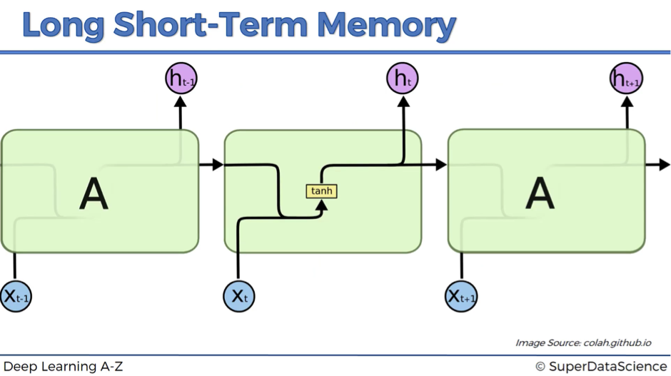
So, the first image below demonstrates how a standard RNN looks like from the inside.
The hidden layer in the central block receives input xt from the input layer and also from itself in time point t-1, then it generates output ht and also another input for itself but in time point t+1.
This is a standard architecture that doesn’t solve a vanishing gradient problem.
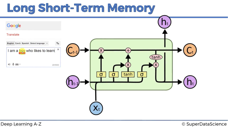
The next image shows how LSTMs look like.
This might seem very complex at the beginning, but don’t worry!
We’re going to walk you through this architecture and explain in detail, what’s happening here.
By the end of this article, you’ll be completely comfortable with navigating LSTMs.
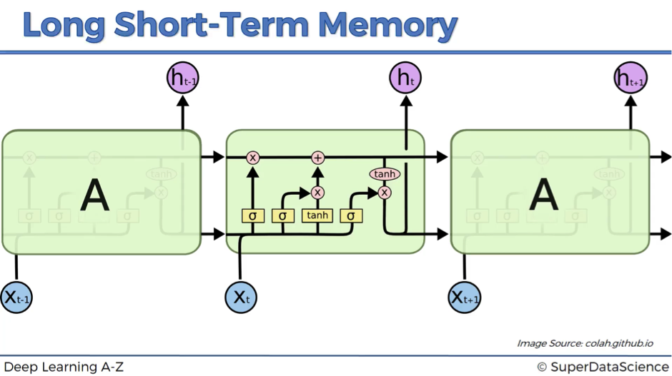
As you might recall, we’ve started with the claim that in LSTMs wrec = 1. This feature is reflected as a straight pipeline on the top of the scheme and is usually referenced as a memory cell. It can very freely flow through time. Though sometimes it might be removed or erased, sometimes some things might be added to it. Otherwise, it flows through time freely, and therefore when you backpropagate through these LSTMs, you don’t have that problem of the vanishing gradient.
Notation
Let’s begin with a few words on the notation:
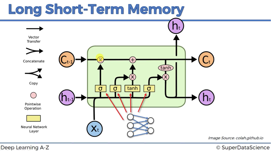
- ct-1 stands for the input from a memory cell in time point t;
- xt is an input in time point t;
- ht is an output in time point t that goes to both the output layer and the hidden layer in the next time point.
Thus, every block has three inputs (xt, ht-1, and ct-1) and two outputs (ht and ct). An important thing to remember is that all these inputs and outputs are not single values, but vectors with lots of values behind each of them.
Let’s continue our journey through the legend:
- Vector transfer: any line on the scheme is a vector.
- Concatenate: two lines combining into one, as for example, the vectors from ht-1 and xt. You can imagine this like two pipes running in parallel.
- Copy: the information is copied and goes into two different directions, as for example, at the right bottom of the scheme, where output information is copied in order to arrive at two different layers ht.

- Pointwise operation: there are five pointwise operations on the scheme and they are of three types:
- “x” or valves (forget valve, memory valve, and output valve) – points on the scheme, where you can open your pipeline for the flow, close it or open to some extent. For instance, forget valve at the top right of the above scheme is controlled by the layer operation s. Based on a decision of this sigmoid activation function (ranging from 0 to 1), the valve will be closed, open or closed to some extent. If it’s open, memory flows freely from ct-1 to ct. If it’s closed, then memory is cut off, and probably new memory will be added further in the pipeline, where another pointwise operation is depicted.
- “+” – t-shaped joint, where you have memory going through and you can add additional memory if the memory valve below this joint is open.
- “tanh” – responsible for transforming the value to be within the range from -1 to 1 (required due to certain mathematical considerations).
Neural Network Layer: layer operations, where you’ve got layer coming in and layer coming out
Walkthrough the architecture
Now we are ready to look into the LSTM architecture step by step:
- We’ve got new value xt and value from the previous node ht-1 coming in.
- These values are combined together and go through the sigmoid activation function, where it is decided if the forget valve should be open, closed or open to some extent.
- The same values, or actually vectors of values, go in parallel through another layer operation “tanh”, where it is decided what value we’re going to pass to the memory pipeline, and also sigmoid layer operation, where it is decided, if that value is going to be passed to the memory pipeline and to what extent.
- Then, we have a memory flowing through the top pipeline. If we have forget valve open and memory valve closed then the memory will not change. Otherwise, if we have forget valve closed and memory valve open, the memory will be updated completely.
- Finally, we’ve got xt and ht-1 combined to decide what part of the memory pipeline is going to become the output of this module.
That’s basically, what’s happening within the LSTM network. As you can see, it has a pretty straightforward architecture, but let’s move on to a specific example to get an even better understanding of the Long Short-Term Memory networks.
Example walkthrough
You might remember the translation example from one of our previous articles. Recall that when we change the word “boy” to “girl” in the English sentence, the Czech translation has two additional words changed because in Czech the verb form depends on the subject’s gender.

So, let’s say the word “boy” is stored in the memory cell ct-1. It is just flowing through the module freely if our new information doesn’t tell us that there is a new subject.
If for instance, we have a new subject (e.g., “girl”, “Amanda”), we’ll close the forget valve to destroy the memory that we had. Then, we’ll open a memory valve to put a new memory (e.g., name, subject, gender) to the memory pipeline via the t-joint.
If we put the word “girl” into the memory pipeline, we can extract different elements of information from this single piece: the subject is female, singular, the word is not capitalized, has 4 letters etc.
Next, the output valve facilitates the extraction of the elements required for the purposes of the next word or sentence (gender in our example). This information will be transferred as an input to the next module and it will help the next module to decide on the best translation given the subject’s gender.
That’s how LSTM actually works.
Additional reading
First of all, you can definitely reference the original paper:
- Long Short-Term Memory by Sepp Hochreiter and Jurgen Schmidhuber (1997).
Alternatively, if you don’t want to get that deep into mathematics, there are two great blog posts with very good explanations of LSTMs:
- Understanding LSTM Networks by Christopher Olah (2015)
- Understanding LSTM and its diagrams by Shi Yan (2016)
That’s it for LSTM architecture. Hopefully, you are now much more comfortable with this advanced deep learning topic. If you are looking for some more practical examples of LSTM’s application, move on to our next article.