Convolutional Neural Networks (CNN): Step 4 – Full Connection

(For the PPT of this lecture Click Here)

---

As you see from the image below, we have three layers in the full connection step:

• Input layer
• Fully-connected layer
• Output layer

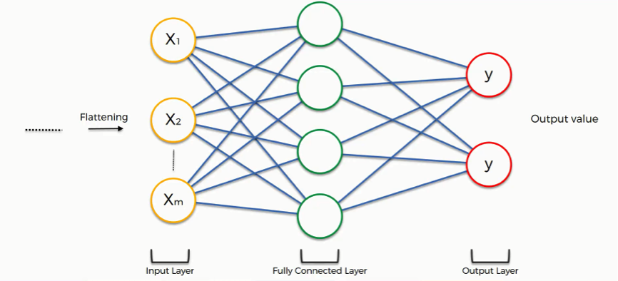
Notice that when we discussed artificial neural networks, we called the layer in the middle a “hidden layer” whereas in the convolutional context we are using the term “fully-connected layer.”

As we said in the previous tutorial, the input layer contains the vector of data that was created in the flattening step. The features that we distilled throughout the previous steps are encoded in this vector.

At this point, they are already sufficient for a fair degree of accuracy in recognizing classes. We now want to take it to the next level in terms of complexity and precision.

The role of the artificial neural network is to take this data and combine the features into a wider variety of attributes that make the convolutional network more capable of classifying images, which is the whole purpose from creating a convolutional neural network.

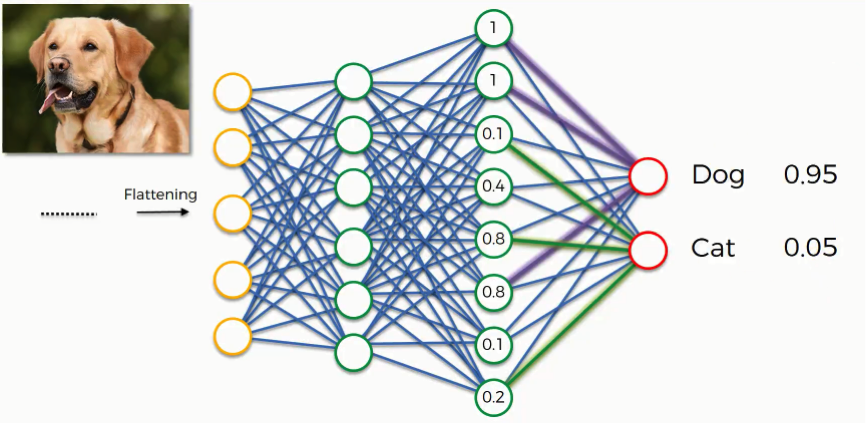
We can now look at a more complex example than the one at the beginning of the tutorial.

We’ll explore how the information is processed from the moment it is inserted into the artificial neural network and until it develops its classes (dog, cat).

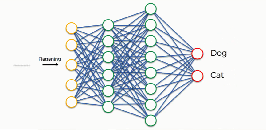
At the very beginning, as you know by now, we have an input image which we convolve, pool, flatten, and then pass through the artificial neural network.

By the end of this channel, the neural network issues its predictions. Say, for instance, the network predicts the figure in the image to be a dog by a probability of 80%, yet the image actually turns out to be of a cat. An error has to be calculated in this case.

In the context of artificial neural networks, we call this calculation a “cost function” or a mean squared error, but as we deal with convolutional neural networks, it is more commonly referred to as a “loss function.” We use the cross-entropy function in order to achieve that.

The cross-entropy function and mean squared errors will be discussed in detail in a separate tutorial, so, if you’re interested in the topic, you can stick around for the extra tutorials at the end of this section.

For now, all you need to know is that the loss function informs us of how accurate our network is, which we then use in optimizing our network in order to increase its effectiveness. That requires certain things to be altered in our network.

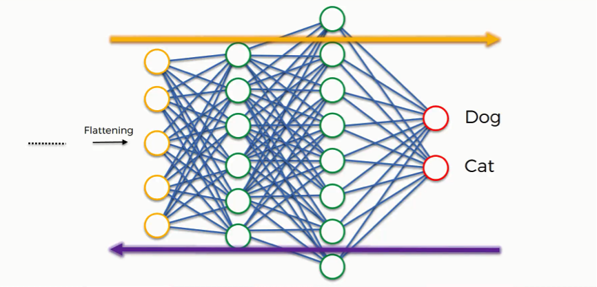
These include the weights (the blue lines connecting the neurons, which are basically the synapses), and the feature detector since the network often turns out to be looking for the wrong features and has to be reviewed multiple times for the sake of optimization.

Just as we said when discussing artificial neural networks, the information is then conveyed in the opposite direction as you see in the figure below. As we work to optimize the network, the information keeps flowing back and forth over and over until the network reaches the desired state.

As you’re always reminded, this process is explained here in an intuitive manner, but the science and the mathematics behind it are more complex, of course.

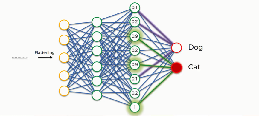
Up until now, we’ve been discussing examples where the output consists of a single neuron. Since this one contains two, there are some differences that show up. Let’s first look at the “dog” class.

In order to understand how it will play out, we need to check out the weights placed on each synapse linking to this class so that we can tell which attributes/features are most relevant to it.

This full connection process practically works as follows:

• The neuron in the fully-connected layer detects a certain feature; say, a nose.
• It preserves its value.
• It communicates this value to both the “dog” and the “cat” classes.
• Both classes check out the feature and decide whether it’s relevant to them.

In our example, the weight placed on the nose-dog synapse is high (1.0), which means that the network is confident that this is a dog’s nose.

Since the information is constantly flowing in both directions, the “cat” class takes note of this and understands that since this is a dog’s nose, then it simply can’t be a cat’s nose. Even if at first it would have considered the signal saying “small rounded nose” because this might be a cat’s as well as a dog’s nose, now it dismisses this feature.

This happens gradually as it receives the same reading multiple times. The dog class on its part will start focusing more on the attributes carrying the highest weight (the three thick purple lines), and it will ignore the rest.

The same process simultaneously occurs with the cat, enabling it to pick out its own priority features. What we end up with is what you see in the image below. As this process goes on repeat for thousands of times, you find yourself with an optimized neural network.

The next step becomes putting our network’s efficacy to the test.

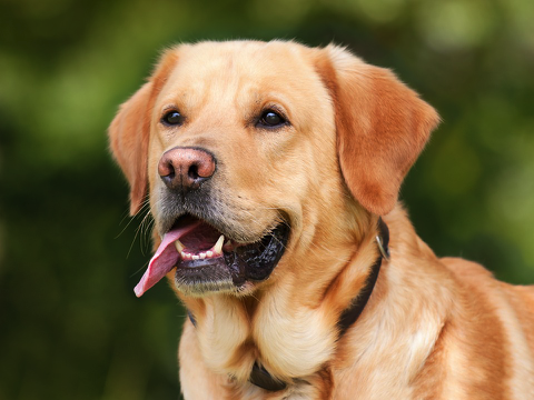
Say, we give it an image of a dog.

The dog and cat classes at the end of the artificial neural network have absolutely no clue of the image. All they have is what is given to them by the previous layer through the synapses. By now, each of these classes has three attributes that it’s focusing its attention on.

That previous layer passes on which of these features it detects, and based on that information, both classes calculate their probabilities, and that is how the predictions are produced.

As you see in the step below, the dog image was predicted to fall into the dog class by a probability of 0.95 and other 0.05 was placed on the cat class.

Think of it this way: This process is a vote among the neurons on which of the classes the image will be attributed to. The class that gets the majority of the votes wins. Of course, these votes are as good as their weights.

Remember this image?

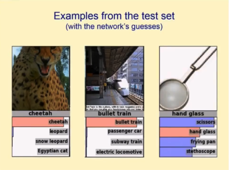
We saw this example in the first tutorial in this section, and by now you have an understanding of the whole process by which these guesses were produced.

Continue with Summary by Clicking Here