

How do Neural Networks Learn?
(For the PPT of this lecture Click Here)

Now we have seen Neural Networks in action it is time to get into deep learning on how they learn.
There are two fundamentally different approaches to getting the desired result from your programme.
Hardcoding
This is where you tell the programme specific rules and outcomes, then guide it throughout the entire process, accounting for every possible option the programme will have to deal with. It is a more involved process with more interaction between the programmer and programme.
The other approach is what we have been studying so far.
Neural Networking
With a Network, you create the facility for the programme to understand what it needs to do independently. You provide the inputs, state the desired outputs, and let it work its own way from one to the other.
The difference between these approaches is as follows. Hardcoding is the man driving his car from one point to another, using road signs and a map to navigate his own way to his destination. Neural Networking is a self-driving Tesla.
Let’s revisit some old ground before we plow into fresh earth
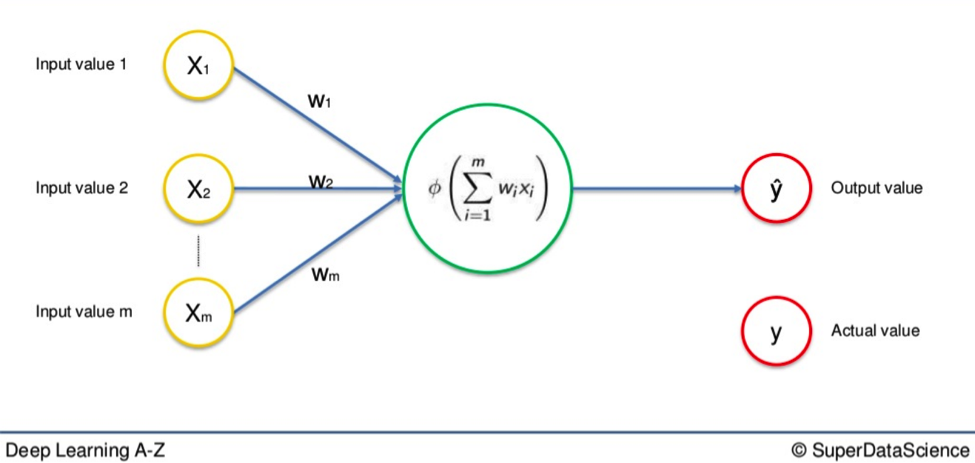
Here is a basic Neural Network we have seen many times so far in these tutorials.
You have the single row of input variables on the left. The arrows that represent weighted synapses go into the large neuron in the middle. And on the right, you have the output value. This is called a Single-Layer Feedforward Neural Network. As you can see, the output value above is represented as Y. This is the actual value.
We are going to replace that with Ŷ, which represents the output value.
The difference between Y and Ŷ is at the core of this entire process.
When input variables go along the synapses and into the neuron, where an activation function is applied, the resulting data is the output value, Ŷ.
In order for our Network to learn we need to compare the output value with the actual value.
There will be a difference between the two.
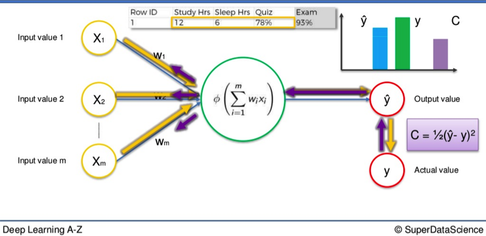
The Cost Function
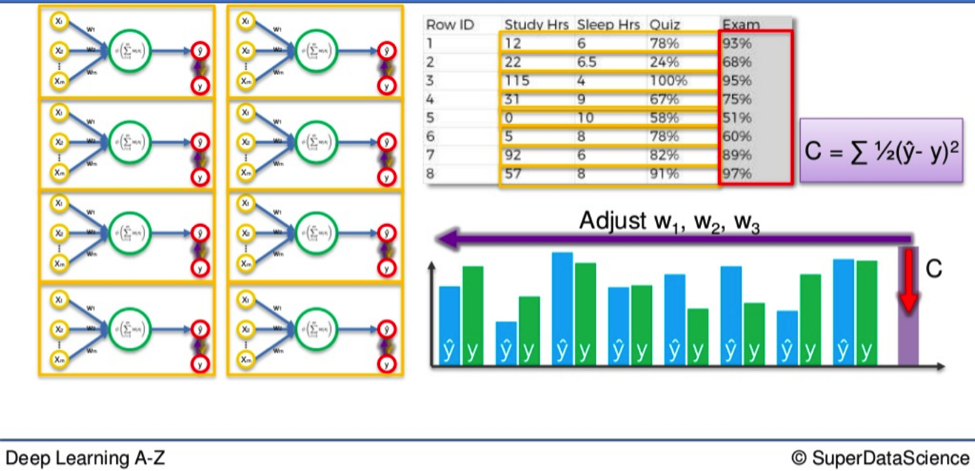
Then we apply what is called a cost function (Cost function – Wikipedia), which is one half of the squared difference between the output value and actual value. This is just one commonly used cost function. There are many. We will apply this particular one in our calculations.
The cost function tells us the error in our prediction.
Our aim is to minimize the cost function. The lower the cost function, the closer Ŷ is to Y, and hence, the closer our output value to our actual value. A lower cost function means higher accuracy for our Network. Once we have our cost function, a recycling process begins.
We feed the resulting data back through the entire Neural Network. The weighted synapses connecting the input variables to the neuron are the only thing we have any control over.
As long as there exists a disparity between Y and Ŷ, we will need to adjust those weights. Once we tweak them a little we run the Network again. A new cost function will be produced, hopefully, smaller than the last.
Rinse and Repeat
We need to repeat this until we scrub the cost function down to as small a number as possible, as close to 0 as it will go.
When the output value and actual value are almost touching we know we have optimal weights and can therefore proceed to the testing phase, or application phase.
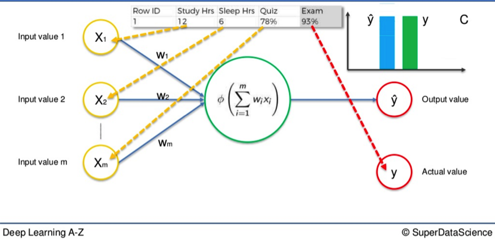
Example
Say we have three input values.
- Hours of study
- Hours of sleep
- Result in a mid-semester quiz
Based on these variables we are trying to calculate the result in an upcoming exam. Let’s say the result of the exam is 93%. That would be our actual value, Y.
We feed the variables through the weighted synapses and the neuron to calculate our output value, Ŷ.
Then the cost function is applied and the data goes in reverse through the Neural Network.
If there is a disparity between Y and Ŷ then the weights will be adjusted and the process can begin all over again. Rinse and repeat until the cost function is minimized.
In this example that would mean our output value would equal the actual value of the 93% test score.
Remember, the input variables do not change.
It is only the weight of the synapses that alters after the cost function comes into play. To give you an idea of the potential scope of this process we can extend this example. The simple Neural Network cited above could be applied to a single student.
Go Bigger
What if you wanted to apply this process to an entire class? You would simply need to duplicate these smaller Networks and repeat the process again.
However, once you do this you will not have a number of smaller networks processing separately side-by-side.
They actually merge to form a single, much larger Neural Network.
So when you again go through the process of minimizing the difference between Y and Ŷ for an entire class, the cost function phase at the end will adjust for every student simultaneously.
If you have thirty students the Y / Ŷ comparison will occur thirty times in each smaller network but the cost function will be applied to all of them together.
As a result, the weights for every student will be adjusted accordingly, so on and so forth.
Additional Reading
For further reading on this process, I will direct you towards an article named A list of cost functions used in neural networks, alongside applications. CrossValidated (2015).
I hope you found something useful in this deep learning article. See you next time.